Introduction

Throughout this chapter, several factors of education and inequality are discussed beginning with the rising costs of higher education and the contribution to the college debt crisis. Stemming from the college debt crisis, there is a connection between one’s level of wage and one’s level of education. Differences in educational attainment lead to increasing educational inequality and income inequality. The college debt crisis has led to rising tuition costs and higher student debt. This increase in student debt has had a major impact on the educational value and on the returns to schooling for students attending higher education. The return to education has several factors influencing the result, two major components are the supply and demand of college educated workers and the human capital bestowed in the laborers. These factors determine the wages desired by individuals and guide their decisions in education. There are many factors influencing educational inequality, and income is one of the most powerful predictors for children’s educational attainment. Some income based demographics and other factors would affect educational inequality, but they all include income in some way.

1.1 The Rising Costs of Higher Education

“The real cost of higher education per full-time equivalent student has grown substantially over the last 75 years, and the rapid rise since the early 1980s is a cause of considerable public concern” (Archibald, Feldman, 2008). Knowing that higher education costs have become a topic of discussion, it is important to note and inspect the actual costs of higher education, the opportunity costs, the cause of rising costs, and future policy changes moving towards affordability and attainability.

1.1.1 Cost Disease Theory

Historically, there are two competing approaches to explain rising higher education costs; cost disease and revenue theory. The theory of cost disease, originally developed by William G. Bowen (1966) and Baumol (1967), creates the idea that there is a constraint faced by colleges. It also suggests that the relative cost of education rises because the rate of productivity growth in this sector is lower than in many others (Archibald, Feldman, 2008). As innovation occurs, workers produce more output across various sectors of the economy, therefore raising wages. However, not all sectors are able to innovate and economize labor as wages rise. Because of this constraint, prices rise to cover extra labor costs.

The figure below illustrates another concept of the cost disease theory; that provided the existing technology, a college can only increase quality with an increase in costs per unit. Therefore, an institution would choose its point on the constraint below given its revenue. Because of this, without an increase in costs and increased revenue, quality will decrease over time. Therefore, institutions will increase prices in order to increase revenue and retain or improve quality. Without improvements in technology, the cost disease phenomenon will lead to rising prices.

1.1.2 Revenue Theory of Cost

A competing theory is the revenue theory of cost originally developed by Howard Bowen (1965). Using the same constraint graph shown above, Bowen theorized that given the revenue constraint, rather than increasing prices, institutions would attempt to loosen the constraint. Colleges and universities want increasing quality, but the expense of losing potential students due to increasing costs will sometimes outweigh the quality gains. Bowen’s revenue theory of cost developed around the idea that colleges and universities are concerned with quality as well as “educational excellence, prestige, and influence” that attracts future applicants. Because of this conflict, institutions do not want to raise revenue to improve quality at the expense of the “educational excellence, prestige, and influence,” that attracts potential students (Archibald, Feldman, 2008).

1.1.3 The Real and Opportunity Costs of Higher Education

Generally speaking, economists have agreed that higher education-specific explanations like Bowen’s revenue theory are less effective at explaining the rising costs of education compared to the cost disease theory. However, other economists turn to data to pinpoint the cause of increasing costs. In a Pew Research study conducted in 2014, economists measured the value of a college education, the decreasing value of a high school diploma, and the rewards and penalties associated with obtaining a higher education.  The main conclusion was that college-educated workers entering the job market are more likely to be unemployed, and their job search will be longer (Taylor, et. al, 2014). However, once they find employment, their earnings will be higher than earlier college-educated workers. When college-educated workers are entering the workforce, they are more likely to face a longer job search due to increased market competition and volume. Because college-educated workers earn a higher income after employment, there is an increase in demand for college education. Even higher tuition rates and attendance costs cannot dissuade potential college students who observe the increasing return to higher education. As a result, the cycle repeats. Demand for college education grows, the number of college-educated workers increases while the period of unemployment lengthens, and tuition costs and college debt continue to rise (Taylor, et. al, 2014).

As a result of the disparity between educated versus uneducated workers and earlier versus newer educated workers, there is an increase in demand for higher education. As the demand grows, universities, especially private or highly competitive, have a limited supply to provide. Therefore, the costs will increase to provide the same quality of education for more, select students, as well as housing and other associated fees. This is indicative of the cost disease theory that quality must continue to increase and therefore, revenue and costs (Archibald, Feldman, 2008).

1.1.4 The Role of Government Funding

A more direct result of increasing educational costs could be due to government funding. Government subsidies for a good or service naturally affect the behavior of both suppliers and demanders. In the case of higher education, as college becomes more costly, government subsidies and aid will increase, and there is a change in demand. As college becomes more affordable due to subsidies, the reduction in price causes a shift along the demand curve (Archibald, Feldman, 2012).  This feeds into the increasing demand for higher education mentioned above. And as the demand shifts, the number of students will increase, as will the costs to provide the same quality to a larger quantity. Therefore, as government subsidies and aid increase, there will be a shift along the demand curve, costs will increase, and subsidies and aid will need to increase once again. This creates a cycle of increasing costs.

Government funding directly influences what universities charge for attendance. More indirectly however, changes in government funding also modify universities’ own resource allocation decisions. Because of this, levels of research effort and prices of resources for instruction can change (Archibald, Feldman, 2012).

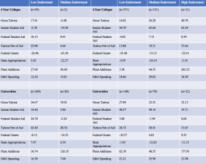
The data below found that while there is a difference in spending and costs between the private and public sectors, there is a correlation between government funding and tuition rates, especially in the public sector. Because institutions in the public sector are typically more dependent on government subsidies, the effect on tuition is much larger than that of the private sector. The data supports the conclusion that in the private sector, net tuition has risen less rapidly than spending. It can also be concluded that in the public sector, where institutions are more reliant on government funding, their spending per student has risen more slowly and their net tuition revenues have grown more rapidly (McPherson, et. al, 1989). This can be supported by a 2014 study done in Virginia. The researchers concluded that in 2011-2012, of the 50 states, 49 spent less per undergraduate student than before the Great Recession, and 29 states decreased per-student funding by more than 25% since the financial crisis of 2007-2008 (Mulhern, et. al, 2015).

Using the data below from McPherson’s study, an econometric model was developed. In this model, universities are institutions with goals and a budget constraint. Given government funding, the institution has to decide how to allocate resources. Any findings using this model will help develop a better understanding of the behavior and resource allocation of colleges and universities and guide future policies (McPherson, et. al, 1989).

1.1.5 The Future of Higher Education

While the rising costs of education is evident, it stems from a variety of sources whether it is government subsidies, or the effects of supply and demand due to economic benefit and increased reward, or the cost disease model. Understanding the future of higher education and the impact of continuous rising costs is important to guiding future policy decisions and debates. Higher education is undeniably the key to future success, financial stability, and inevitably innovation and prosperity. Without addressing the causes of rising costs, it is impossible to guide future policies and make education both affordable and attainable for the betterment of our future innovation and prosperity.

Among economists, there is a general consensus that the lack of affordability of public colleges and universities will impact gaps in income inequality and socioeconomic status. Currently in Virginia, economists Mulhern, Spies, Staiger and Wu note that higher education has become less financed by state appropriations and more from tuition. Because of this, institutions are more dependent on tuition revenue for resources. In order to pay salaries, scholarships, financial aid and other resources, institutions will increase tuition. This consistent decrease in state funding, and thus increase in tuition will only decrease educational attainment and affordability (Mulhern, et. al, 2015).

Using Virginia as a specific study allows economists and researchers to draw specific conclusions that can be applied to the remaining 49 states experiencing similar conflicts. It seems that the reduction in state funding and increase in tuition creates a revolving cycle that serves only to make higher education less attainable and affordable, especially following the financial crisis that began in 2007. Nationally, as of 2012, only 42% of 24-35 year olds had a post secondary degree. Even more discouraging, students from upper-income families with at least one college educated parent were eight times more likely to obtain a college degree compared to those from low-income households without college educated parents. Both statistics given are proof of the stark difference in educational attainment for students of different socioeconomic statuses (Mulhern, et. al, 2015).

It is obvious that socioeconomic status has an effect on educational attainment, and educational attainment has an effect on income. Because of this relationship, there is an increasing demand for higher education. With this increase in demand comes an increase in costs to provide the same quality to a larger quantity. As costs increase, as does the difficulty to acquire higher education. This cycle creates a problem for states and institutions. They face a constraint, where increasing costs increases the opportunity gap between students from different classes and where decreasing costs lowers quality. Knowing this constraint exists, states have made attempts to increase the number of college educated graduates and decrease the opportunity gap between socioeconomic groups (Mulhern, et. al, 2015). However, reductions in state appropriations threatens enrollment levels and increases the opportunity gap. Even with policy changes and attempts at managing this cost constraint, higher education costs continue to grow, especially for lower income students (Mulhern, et. al, 2015).

The various failed efforts at controlling rising costs and opportunity gaps implies that the current educational funding in the United States cannot be repaired or reversed, but must be rewritten entirely. This research and data suggests one main point: our education system is flawed, and new policy decisions and debates must occur to change the future of higher education. To summarize the issue, “Rising costs and increasing financial pressures on public colleges and universities across the nation threaten to lower overall educational attainment levels and magnify gaps in income inequality and socioeconomic status” (Mulhern, et. al, 2015). Knowing that higher education impacts wages, earnings and future financial stability increases the demand for higher education. While this increase in demand is occurring, education is becoming more unattainable and unaffordable. Our economy would serve to benefit from a growing number of increased individuals joining the workforce, however the growing gap in income inequality and educational attainment is deterring and slowing the economic growth provided by increased education (Mulhern, et. al, 2015).

It is most important to understand that there is a constant rising cost of higher education that will permanently affect the future workforce and the overall economy due to lower educational attainment levels and affordability. The rising cost of higher education contributes greatly to the college debt crisis and its effects, wage differences in the workforce, and inequality in both education and income.

1.2 College Debt Crisis

After the financial crisis, students have been dealing with the backlash of having rising tuition costs which have been affecting them both during their college years and after. There have been many studies done examining the correlation between the college financial crisis and education. These studies have ranged from looking into the return to schooling of these students, to seeing if these students would be able to pay off their student debt at any point in their lives. This includes many students believing that they won’t be able to have families and careers. Graduates with high amounts of debt have been found to be less satisfied with their work, work more, and were less likely to work in a field relating to their major (Velez,2019). Having all of these studies allows for great insight into whether or not the higher education system in the U.S. is actually worth attending anymore. Students believe that attending college hasn’t been worth it, since they may attain huge amounts and debt and may not be able to pay them off in time to see returns to their schooling until it’s too late. The fear of failing and not being able to have a successful life is affecting a lot of students. They understand that for most of them, the burden isn’t just held by themselves alone. Their parents are also paying off some of their debt, in the cases of students that weren’t able to attain scholarships. A combination of many of these different things while attending college has driven many students’ academic performances downward. Most of these studies all agree with the same conclusion; that attaining massive debt and having a lack of financial knowledge is greatly correlated with students’ poor academic performance.

1.2.1 Government Spending in Colleges

After the Great Recession finally passed, and the financial market started to recover, the U.S. Government was still in great trouble, since they couldn’t recover as quickly. This led to many cuts in the budgets of funds to public universities. Government spending on college funds was down ~$9 Billion after in 2017 from 2008, after adjusting for inflation (Mitchell, 2017). Out of every state, 44 out of the 49 studied from 2008 until 2017 spent less on students (Mitchell, 2017). These states ranged from Arizona ,spending 53.8% less on their students, to Maryland which only spent .8% less (Mitchell, 2017). States have started to try and reverse these cuts in more recent years once they realized just how quickly student debt was rising. 36 out of the 49 states mentioned earlier increased spending in 2016-2017, but only on average of $170 (Mitchell, 2017). Even though many states have tried to increase spending, their efforts haven’t been able to offset the cuts that occurred as a result of the Great Recession. These cuts forced many public universities to have higher tuition costs since they still had to maintain the status of the university. Without those government funds the costs that were associated with the day-to-day running of the school had to be transferred over to the students. This included paying for faculty, maintenance workers, student meals, etc. Students have been paying progressively more and more in tuition to help keep public universities intact. In 2016, over half of states had student tuition exceed their state and local government funding for schooling. It has gotten to the point where in 9 states, tuition is double what they are receiving in government aid (Mitchell, 2017).

1.2.2  Rising Tuition

Annual tuition in public universities has risen by 35% and in some states has led to increases by up to 60% in multiple states (Mitchell, 2017). This was a great contributor to the start of the U.S. college debt crisis. Many students quickly realized that their tuition bills were rapidly rising. By raising college tuition by so much, some incoming students decided that school may not be the correct option for them. This was for a plethora of reasons. Firstly, some of these students just weren’t able to afford the tuition. This was even unaffordable for them with the help of their parents’ income. “Between 1973 and 2015, average inflation-adjusted public college tuition has risen by 281 percent, while median household income has grown by only 13 percent” (Mitchell, 2017). Tuition has risen by enough to even outpace the top class of families. “Over this period, the incomes of the top 1 percent of families have grown by about 186 percent. This means that public college tuition has outpaced income growth for even the highest earners” (Mitchell, 2017). This has forced many low income students to make the decision to not attend college since it wouldn’t be worth it for them to attend since they couldn’t keep up with the payments even with financial aid. “In 2015, 58 percent of recent high school graduates from families with income in the lowest 20 percent enrolled in some form of postsecondary education, compared to 82 percent of students from the top 20 percent” (Mitchell, 2017). This gap has grown significantly from years past.  Some students even received scholarships and it was shown that by attending public universities they received lower amounts than their peers who attended private schools. Students with lower income haven’t been able to keep up with these rising costs; forcing them to take out more loans that put them further into debt. “Pell Grant recipients must have a family income under $50,000 to be eligible to receive the grant.” Many students, since their income is so low, have very little options to be able to pay off rising tuition costs and may not be able to reach out to family to help pay off these loans as discussed in previous sections. “A full 84 percent of graduates who received Pell Grants graduate with debt, compared to less than half (46%) of non-Pell recipients” (Huelsman, 2015). The Gates Millennium Scholars Program offered $1 Billion over a 20 year span to low income, high achieving minority students. It was designed to help promote academic achievements and to offer these students a chance at higher education while allowing them to have less debt. Students that went to public universities received around $8,000, while private school attendees received $11,000 (DesJardins, 2014). The GMS Program and Pell Grants still haven’t been able to offset the rise in tuition. Having to take out more loans also forces lower income students to make the choice of attending college at all or taking a smaller amount of classes to be able to manage their debt. For every 10% increase in student loans, it was seen that took half a credit less. Freshman with loans were also 3% less likely to return to school (Stoddard, 2018). Many students are becoming skeptical now of enrolling in college, since they now believe that even if they do enroll, that they will amass a debt so large that they won’t be able to do many of the things that they aspire to do in life. This includes, starting a family, raising their net worth and savings, as well as being able to own a home. Students have started to realize that while attending college for longer and amassing larger and larger amounts of debt, it lowers their net lifetime earnings. The students who still choose to enroll have also been seen to have much higher stress levels now. This has been happening since many of them have been worried about all of the same things that were mentioned before, but the only difference is that they are also taking on this massive amount of debt while trying to pass the courses that they are taking. ”Additionally, health professions students and graduates experience susceptibility to personal risks (psychological distress, burnout, decreased quality of life, and decreased satisfaction with work-life balance, among others) associated with educational debt, which may worsen should debt-to-income ratios increase” (Chisholm-Burns, 2019). This increase in stress has also been attributed to the increase in rising tuition, especially for medical students. “Among medical school graduates in 2018, more than 70% had student loans for medical school, and more than one quarter had student loans totaling between $200,000 and $299,000” (Chisholm-Burns, 2019). The GMS grant mentioned above, helped to decrease the amount of stress that these students were going through. The study showed that these students’ hours worked per week dropped significantly, as well as the amount of debt these students took on. The study proved that by having this burden lightened and allowing for these students to focus more on their studies that their GPAs were raised and that they did better on tests as well. Scholarships have been used to lessen the burden on these students and have them amass smaller amounts of debt, but it hasn’t been enough to offset the amount that these students have to pay in tuition. There is a correlation between students’ borrowing on non-loan aid vs loan aid as well.  Students that borrowed gained 0.1 points onto their GPAs; but it was found that a 10% increase in their loans relative to their tuition costs actually reduced their GPAs by 0.4 points. (Stoddard, 2018). Having a slight increase in tuition can actually raise GPAs, but as that loan number increases it actually becomes harmful to the student. When non-loan aid, such as scholarships or Pell grants as discussed above, were introduced, students performed much better and saw a rise in their GPAs. “…for students who receive Pell grants in some semesters but not in others, their GPAs are 0.05 points higher in the Pell aid semesters” (Stoddard, 2018).

1.2.3 Parents Income

Many students at the end of the Great Recession thought that enrolling in college would be a great idea, since many of the markets would be in a trough and would be looking for skilled workers. This would lead to them having a much greater chance at achieving higher wages and having their dream life. Between 2005-2011, 39.9% of 18-24 year olds enrolled in college, which was an 11.1 percentage point increase since 1985 (Faber, 2018).  The problem was that since government spending had hit an all time low in college spending since they didn’t have revenue due to the collapse of many financial institutions, students didn’t foresee the greatly increased college tuition fees. Many students only realized this once they had already enrolled in college. Parents saw these increased prices and started to increase their spending in their childrens’ college tuition costs. Parents were seen covering roughly 45% of their childrens’ loans, with that number increasing as family income increased as well (Faber, 2018). Parents still believed that they could make enough money to cover all of these costs. The problem was that income wasn’t rising fast enough to cover these costs. From 1973 to 2015, tuition costs have risen by 281 percent, while income only rose by 13 percent (Mitchell, 2017).  Many of these parents didn’t realize just how much the popping of the housing bubble, as well as the collapse of financial institutions, had also increased the amount of mortgages. They quickly realized that they weren’t able to keep up with the increased tuition costs as well as keep up with their mortgage payments. This forced the parents to have to foreclose on their homes. It was shown that with every 1% increase in college attendance there were roughly 19,000 foreclosures that occurred (Faber, 2018). Having these foreclosures occur, many students started to feel pressured and started to take out loans themselves to make it much easier on their parents. This was a great contributor to many students’ college debt and academic studies. Students started to feel the pressure of school, while trying to make the most out of their education since they had this sense of massive failure if they didn’t proceed to graduate on time, pay off their loans as quickly as possible and save their families futures.

1.2.4 Return to Schooling

Many students are very unsure as to how their future’s will end up with all of this debt that they amass during college. High school students looking to attend college coming from lower income families don’t look into selective colleges, such as Harvard and Yale due to the debt factor. “A large share of high-achieving students from struggling families fail to apply to any selective colleges or universities, a 2013 Brookings Institution study found. Even here, research indicates that financial constraints and concerns about costs push lower-income students to narrow their list of potential schools and ultimately enroll in less-selective institutions.”(Mitchell, 2017). Many students are also unsure about their experiences and feel as though they have had a much lower quality of education during their college years. This is due to the massive cuts that the institutions have made, despite raising tuition costs greatly. Institutions have cut faculty members, courses, and even complete majors to try and keep themselves going. By having fewer classes, while having more students enroll, many of them believe that they aren’t going to see the return to schooling that they were hoping for. Students believe that their education has left them unprepared for what is to come later in life. Feeling unprepared and having massive amounts of debt, they fear that they will have lower paying jobs and it will take them much longer to pay off their debts. This was proven in a study that simulated college students’ debts and earnings over the years. It was found that students who went to college in STEM fields and business majors made more money than their counterparts. The problem was that even though many of these students found themselves making more money, they had a small premia on their return to schooling. They found that the premia for STEM/Business majors was ~$220,000 after accounting for debt taken in from student loans, ~$30,000 per year, and costs not associated with student loans, ~$7,000, on average (Webber, 2016). Students that would attend for Arts/Humanities were found to not have a premia at all anymore. This was because they accounted for a variable that most other studies omitted, which was the ability factor. The study used the upper bound of this as the 25th percentile, because once the ability factor was introduced, there was drastic heterogeneity within the majors themselves. It was found that at the 25th percentile, Biology majors were found to have returns to schooling on par with their peers in Arts/Humanities (Webber, 2016), which would make going to college seem not worth it in the long run for them. Economists were only beat out in returns to schooling by a few STEM majors during the study as well (Webber, 2016). They found that many of these students return to schooling not only depended on their ability and how well they did in school but that a major factor was the quality of the institution that they attended.

1.2.5 College Degree Value

Universities have had to make the difficult decision on how to combat the cuts in government spending. It was found that even though tuition rose, universities still had to get rid of faculty and staff. Eastern Illionis had to get rid of over 400 faculty positions, the Kansas Board of Regents eliminated $900,000 in scholarships, and Kentucky Community and Technical College cut over 500 positions, laid off 170 employees, and eliminated 336 positions (Mitchell, 2017). Students enrolled in college were really having doubts about whether to finish college or not since many of them saw their loans as something that lowered their return to schooling and would give them less monetary gains in the future; as well as not receiving a quality education that would prepare them for the future. Younger students are having these same doubts now, since they have seen the massive amount of student debt that has been piling up and don’t want to be trapped in this as well. “Studies suggest that small amounts of debt—$10,000 or below—have a positive impact on college persistence and graduation, but amounts above that may have a negative impact.” (Huelsman, 2015). The main reason many of these students still have trouble deciding on whether or not they want to attend college is because of the fear that they will be one of the few people that won’t be able to pay off their debt in time to be able to live happily. “Households with some college and no education debt have an average of over $10,000 more in retirement savings than indebted households; households with a college degree have over $20,000 more in retirement savings; and dual-headed households with college degrees have nearly $30,000 more in retirement savings.”(Huelsman, 2015). Students have realized that by staying at school for a longer amount of time they are seeing a large drop in their returns to schooling. Students were found to have been able to recover their college costs in 13 years when graduating in 4 years, but it took them 31 years when graduating in 6 years. It showed that students also still had a positive NPV as long as their tuition remained around $26,000/year, with some deviation based on major (Lobo, 2018). This is only for students that amass debt and then finish college to receive their degree. Students have been dropping out of college at much higher rates, while having student loan debt that they will still have to pay off. “The finding that students who take on loans and accumulate more debt are more likely to drop out of school is particularly concerning, as these students will need to meet their loan obligations without earning the higher salaries that result from a college degree” (Stoddard, 2018). Black and Latino borrowers drop out at rates of 65% and 67% respectively at for profit 4 year universities; 47% of black students also drop out of for profit 2 year universities as well (Huelsman, 2015). There are many options to be able to pay off these loans and as the study above showed, as long as they don’t amass a large amount of debt to their name, then they will be able to see returns and monetary gains fairly quickly within their career paths.

1.2.6 Financial Advice

As shown above, many of these students have this notion that going to college may actually be detrimental to their lives, when in-fact it is still helpful. Students thought that with the rising of tuition, that they wouldn’t be able to pay off all of their loans. This fear and stress caused many students’ GPAs to drop.Certain instances of taking on student loans allows for students to increase credits and raise their GPAs, but once loans increase to higher levels then the academic outcomes for students become more adverse  (Stoddard, 2018). This was seen to change once students started to gain knowledge on how to handle their debt. Students realized that once they could actually handle the debt and it wouldn’t deter them from being able to live a full life, their GPAs rose significantly. “More significantly, the intervention increased students’ semester GPAs by 0.077 points” (Stoddard, 2017). This raise in grades showed that many students were only doing worse on exams, because they were so stressed about their future that they couldn’t just focus on their studies. Students also had much more time for school once they figured out that they could attain more scholarships and had many different options to be able to finance their educational loans after they graduated. Students also started to show an increase in retention rates once these letters were given out to them. “The results indicate that the intervention increased retention in the subsequent semester by 1.7 percentage points and in the following year by 5.3 percentage points. This is roughly 2 and 7 percent of mean retention rates (86.5 percent and 78.5 percent) for one semester and one year, respectively” (Stoddard, 2017). By having these letters, students showed that having even a slight increase in knowledge of how they may be able to handle their debt, helps for them to improve academically. Students who do not have this financial knowledge have also been shown to have poorer grades. “Larger loans also reduce retention: among students with loans, those whose ratio of loans to tuition is 10 percentage points greater are 2% less likely to return.” (Stoddard, 2018). Developing an understanding of finances and student loans is extremely important to the academic performance of students and obtaining a higher education degree that will determine their future wage level.

1.3 Wage Differences Between Education Levels

Education is a much needed aspect in all developed and developing countries because it inspires technological changes and provides progression (Fukumura, 2017). Wage differentials arise from changes in supply and demand of workers and education levels resulting in the change of human capital and skilled versus unskilled workers to manipulate wages. There has been an increase in wages yielding a larger return for the more skilled laborers since the 1980’s (Manacorda et al, 2010).

1.3.1 Relationship Between Wages and Schooling

The structure of wages is a concave curve between earnings and years of schooling while also having many other aspects influencing them. Murphy and Welch (1992) explain that individuals who graduated college in 1963 to 1989 made 44% more per hour than high school graduates who did not seek further education. Those same high school graduates earned 35% more per hour than high school dropouts. Throughout their study Murphy and Welch found that education levels across men were increasing through the 60’s until the late 80’s while the return from schooling increased through the 60’s to early 70’s. The return to higher education levels decreased after the switch from the early 70’s up until the early 80’s and then finally increased again from the early 80’s to the late 80’s at a much higher rate than before (Murphy & Welch, 1992). Murphy and Welch expect that the fall in return was related to the population increase from the baby boomers. Throughout the 70’s was when most boomers were entering the labor market because the amount of younger workers was very large. This yielded lower wages causing the 80’s to have the increase in wages as the, before inexperienced, workers have now gained the experience required leading to higher wages (Murphy & Welch, 1992). To explain these turns in wages they examined the GNP for the United States during the same time span and saw about 28% growth from 1963 to 1973. There was also a smaller growth from 1973 to 1989 with only a 1.1 percent growth in GNP. This does correspond fairly well with the results of wages. The reason for the increase in the 80’s was due to the experience of the workers.

Castex and Dechter (2014) explained that declines in returns could be related to differences in the growth rate of technology. The growth rate of technology has shown the relevance of building human capital to make up for times when the growth rate is lower (Castex & Dechter, 2014). If we look at these two studies together, it displays an accurate depiction by explaining the wage levels from 1963-1989. Initially when the GNP was increasing and technology was increasing wages were going up. Next, we see GNP stay relatively the same and wages decreased and then increased again in the early 1980’s due to the increase of human capital from workers throughout the 70’s.

Katz and Goldin (2020) studied the return from college from 1980-2017 with the increase in technology, They examined that the return to college in 2017 was 10.9 log points higher than in 1980. Additionally, they found that the reason for this large college wage premium increase was not entirely to the fault of technological increases such as computers’ and robots’ presence in the workforce, but due to the increase in demand for college educated workers. This is due to the fact that the supply slowed down for several years, but stated that technology could have played a larger role, however, it was unable to be seen with their two factor set-up (Goldin & Katz 2020).

Many believe there are diminishing returns to schooling as said by Colclough, Kingdon, and Patrinos (2010), where we see high returns from primary schooling and lower returns from succeeding schooling. Put simply, this means the more years spent in education increase earnings, but at a lower rate than the initial investment made. Throughout their study they found that the return to primary schooling has been decreasing since the 1950’s. The researchers believe it can be contributed to a supply-side issue and a demand-side issue (Colclough et al, 2010). The amount of people that were completing primary school was increasing at a rate higher than the rate for job creation in many poorer countries, so it became much harder to find a job outside of primary school without receiving more years of schooling (Colclough et al, 2010). As workers saw a decreasing amount in returns, it can be assumed that the private profitability also fell, therefore, decreasing the desire for  primary education. As people see this happening it could cause them to put more stress on secondary schooling in order to increase return. Considering the diminishing returns of education, it is still increasing the overall return just at a smaller rate causing the ongoing years of schooling to be desired in some cases. Recently, a study was done which showed that the return of primary education is much lower now when compared to the return of secondary education. This means that the gap between returns is increasing over time causing schooling to become even more of a necessity. In earlier times, people could get by with only primary education, but since the gap is increasing this may cause people lacking a secondary education to be unable to make ends meet. They are making much less money than an individual that obtained more schooling. (Colclough et al, 2010).

1.3.2 Supply and Demand Factors on Wages

Katz and Murphy explain that the structure of wages is built strongly off of supply and demand of workers including skilled workers, college educated workers, and women workers. They examined the wages of these workers from 1963 to 1989 and saw a 9% increase in relative wages of men and the gender gap during this time did not begin to decrease until the 80’s. During 1963-1989, the college educated workers wages increased by 8% until 1971 when they began to decrease to a point of just over 10% for 8 years and then bounced back in the years following (Katz & Murphy, 1992). The wages increased during this time for college educated workers and women workers while causing the wage inequality to increase as well. Over this same period there was a switch from ordinary industrial manufacturing to more technological jobs causing a larger need for the skilled or college educated workers. This, then, causes a decrease in the demand for primary educated workers and an increase in the demand for secondary educated workers, creating a larger inequality due to wage differentials.

1.3.3 Human Capital and Wage Differences

Human capital when paired with technological change has a large influence on wages argued by Mincer (1991). He refers to the demand for workers when several changes in an industry occur such as when more machines or equipment are bought causing the company to desire more workers to operate them. Additionally, technology advancements have allowed for the company to produce more of a product more efficiently which leads to a lack of workers needed. This is when human capital needs to be acquired by individuals in the job market as the increase in human capital makes them more desirable by a company in order to add value to a product. In an evolving world with many technological advancements, the demand for highly skilled laborers and human capital is much greater than the demand for unskilled laborers causing the wage differential to grow (Mincer, 1991). Increasing human capital can come from higher education, on-the-job training, and years’ experience in a position to lead to higher wages than laborers without these experiences or education. This is due to the difference in productivity of the workers. Laborers with more human capital are seen as more productive than others with less human capital (Mincer, 1991).

During and after a recession, individuals who went to college to build their human capital are oftentimes left in a situation of mismatching in the job market (Liu et al, 2016). Mismatching simply means taking a job that is in a different industry than the industry you specialized in at college. Mismatching is not always bad, if the company that an individual joins outside of his or her specialization allows for upward mobility, then down the line it is potentially worth it. However, if an individual cannot afford to take a low paying job in his or her specialization due to the recession and shortage of jobs available, then they may take a job in another market that will not benefit him or herself in the future. A normal recession is when unemployment rises over 3 percentage points and this causes a possible increase of about 30% chance of mismatching to occur (Liu et al, 2016). So when a country is in a recession, many college students will begin looking for jobs upon graduation and if their industry is hit harder than others, causing a decrease in the demand for workers, the college graduates will need to start looking for jobs in a different industry to start making money. They will find themselves in this situation because many will need to start paying off student loans so the need for money coming in will grow causing them to take jobs outside of their specialization.

1.3.4 Mastering a Trade and Wages

Unions control wages for these skilled jobs which can be a double-edged sword. When unions raise wages, some companies may lay off some of their union workers causing workers to look for jobs in a nonunion section (Western & Rosenfield, 2011). This ultimately lowers the supply of workers so when companies that hire union workers are in higher demand, they are going to have to comply with the larger wages. Throughout the United States many high school students have been encouraged to go to college and get a degree following graduation. This is beneficial as we know more years of schooling increases your return, but at the same time the return has been steadily decreasing. The majority of high school graduates moving on to college rather than mastering a trade has left the trades market short on workers. This has caused individuals seeking a trade skill to have a much higher return as shown by Krupnick (2017).  Krupnick (2017) has quoted Derrick Roberson as saying “All throughout high school, they made it sound like going to college was our only option”. This has led many people steering away from trades such as plumbers, electricians, welders, and many more. It was said in the article that the majority of the workers in these fields currently are over the age of 45 which means they are nearing retirement which will cause an even larger shortage. The demand-side factors of the job market have a large influence on the return and earnings. For example, if the job market is very saturated with people looking for work, the return will be lower than a job that has very few applicants and many firms need a single worker.

1.3.5 Current Job Market and Wages

When we apply these patterns and theories to the current job market, we may notice several things. First, automatic machines in many factories will create a desire for human capital. Second, with many high school graduates going to college and receiving a bachelor’s degree before entering the market, it may cause a saturation of educated workers. Lastly, the demand side of the labor market may be lower due to the pandemic crippling many businesses. As argued by Mincer, there are many technological changes within industries and many operations are becoming automatic in businesses. They will begin to look for individuals with more human capital. This is due to the increased productivity of the equipment that less workers will be desired, allowing the company to focus on the applicants who have more years of experience, more education, and training due to overall human capital from the laborer. Technological advancements and high human capital are complementary to one another by the overall increased productivity. The desire for human capital arises as automated machines begin to be implemented in many manufacturing jobs all over the world, lowering the demand for unskilled laborers increasing the return to skilled laborers. In time, this will cause an increase in supply of human capital due to a high demand for laborers with a high level of human capital.

Years ago many people entered the job market right out of high school while some went on to further their education before entering the market, which ultimately increased the wage difference in individuals. With many high schoolers in today’s era heading to college right after high school, this could cause a saturation in the market lowering the return and people who obtained a master’s degree or higher now are receiving a larger return. This is similar to in the 60’s, when the majority of the laborers had a high school education and the ones making a greater return were college students. Now, when the majority of the laborers have a college degree and the larger return goes to individuals with more years of schooling increasing the overall wage differences.

Lastly, the demand for workers has a large influence on wage differences. As the world is currently in a pandemic, many businesses are operating at a lower production which in turn means they do not need as many workers. If somebody is looking for work, they may have to accept a lower wage decreasing the return to education. This is where mismatching could arise as we see many college students graduating in a recession while the job market is in shambles. Students graduate with a set of skills in the area or field that they majored in having to take jobs in other fields yielding a smaller pay and problems in the long run.

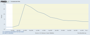
Looking at the  graph above, we see an increase of unemployment jump from sub 5% to over 14%. This will cause a rise in mismatching of college graduates entering the workforce and potentially resulting in those same laborers never switching jobs. Leaving workers out of the field they went to higher levels of schooling for. They found that college students who have their degrees designed for the private sector are much more likely to be affected by the mismatch than graduates who have degrees for the public sector (Liu et al, 2016). If the job market has a low demand for workers in a field that a graduate specialized in, they will then need to search for a job in high demand. Which will have an effect on their return as they are taking a job with limits on the future as their degree and experience may not qualify them for what is needed to progress in that industry. Which in the long run will cause them to have to switch back to the respected industry starting at another entry level position. But, if they stay in the other one they will find themselves stuck at a certain level with very low mobility up within the organization.

1.4. Income Inequality on Education Inequality

The relationship between income inequality and children’s educational attainment and achievement has been a popular research topic around the world. Huge economic growth in the 20th century provided many good opportunities for the parents and children. Between 1947 and 1977, the gross national product per capita doubled. Reardon (2011) and Duncan and Murane (2014) showed that there is an increasing income gap between high-income families and low-income families, even with the incomes for low-income families doubled. As the income inequality is getting bigger, children’s educational attainments and achievements attract more people’s attention.

1.4.1 Relationship between income and education

To analyze the relations between education achievements and income, a worldwide analysis would help to build up a sense to find the relationship between income and education in general. Then, we move to the inside of the US to find out how income and education are related. Worldwide, educational outcomes are positively related to income inequality across countries. In Thorson and Gearhart’s (2018) research, they used the Program for International Student Assessment (PISA) scores from 1980 to 2015 compared with the levels of income inequality across countries. The results indicate that for every one additional percentage of income concentrated in the top 10 percent of the population, which means a larger income inequality, the PISA reading score will be affected between 1.2 points and 3.2 points. The results also suggest that the effect of income inequality has a larger impact on other PISA scores. For every one percentage point increase in inequality, the expected PISA math score decreased between 4.4 points and 7.2 points. The score of the PISA science test follows the same effect from income inequality decreasing between 3.8 points and 5.6 points, which is smaller math, but larger than reading (Thorson & Gearhart, 2018). All the results from the research indicate that there is a positive correlation between income inequality and educational achievement. This relationship also seems to hold within the U.S. for the income inequality and educational attainment and achievement.

In the US, the income has been a huge gap between the high-income families and low-income families, based on the U.S. Census Bureau data, and all of the data we’re using real income, which adjusted the inflation based on 1970. In 1970, the families’ income in the 20th percentile was around 37.7 thousand dollars, and it decreased to around 26.9 thousand dollars in 2010. In contrast, the top richest families, who were in the 95th percentile in 1970, earned about 152.8 thousand dollars, and it increased to 223.1 thousand dollars in 2010.  Moreover, for the families in the 80th percentile, real income increased from about 100.8 thousand dollars to 125.4 thousand dollars from 1970 to 2010. Low-income families’ income was more than 25% lower than in 1970. For the families at the 80th percentile, family income increased by 23%. The income, for the top 5% richest families, increased by 46% (Duncan & Murane, 2014).  It is clear to see that the incomes were increasing at an unequal rate. Based on the real income, the low-income families became even poorer than before, and the very high-income families became even richer. The income gap between high- and low-income families is widening so much, it concludes that richer families are easier to get substantial increases to their income while lower-income households are not.

The education system was experiencing an increase in inequality as long as the increases of income inequality. Reardon (2011) found the gap between the average reading and mathematics skills of students from low-income families and high-income families increased rapidly from the 1970s. In the late 1960s, the gap between the reading and math skills of the wealthiest 10 percent of children and the poorest 10 percent was about 90 points on an 800-point SAT-type scale. After forty years, the gap increased about 50%, nearly 125 SAT-type points (Reardon, 2011). Pfeffer’s (2018) research indicated substantial gaps in educational attainment by family net wealth can be observed across all education levels, including high school attainment, college access, and college graduation. College graduation rates for high-income children expanded from 36% to 54% from 1975 to 1996, in contrast to that, the college graduation rate for low-income students slightly moved from 5% to 9% during the same period (Duncan & Murane, 2014).  Overall, within the United States, it also shows that the gap of educational achievements for low- and high-income families increased with the increase of income gaps. After introducing the relationship between income inequality and educational attainment, we will discuss how rising inequality may influence children’s skills and attainment.

A rising family income inequality would affect children’s skills and attainment from an early age of kids, such as accessing high-quality childcare, schools, and others. It is a growing gap in the resources that low- and high-income families can provide for their children. Wealthy families tend to spend more money on enrichment goods and services to help their children’s education. An increase in parental investment is not only directly affecting the education gap, but it also widens the skill gap indirectly by relating to residential segregation. Residential segregation has been in an increasing trend in recent decades, which means that wealthy families tend to live in some areas with expensive housing and living standards. Low-income families are not able to afford the cost, and that reduces the interaction between low- and high-income families’ children. As a result, the higher quality of schools, child care centers, libraries, and grocery stores are built around the rich neighborhoods. The neighborhood for low-income families may decline in quality including the schools. Children from low-income families could be in a worse scenario from the time they were born (Duncan et. al., 2018).

Meanwhile, low-income families could not afford high-quality child care which helps kids be prepared for kindergarten. That would worsen the starting point for children in low-income families, since children might experience hard-time learning with inattentive classmates. Classes would be harder to teach for teachers as well due to inactive students (Duncan et. al., 2018). Moreover, high-income families are able and tend to spend more on the resources that can help their children’s development. The increasing income inequality widens the spending on children’s enrichment. In 1972-1973, high-income families spent around $2,700 more for each child each year than low-income families. In 2005-2006, the gap of the spending from two families increased to $7,500 (Duncan et. al., 2018). In general, family income has become a strong predictor for college attendance and college quality; each percent increase in income is causing a 0.63 years increase in children’s schooling (Duncan et. al., 2018). Moreover, researchers are considering that “changes in demographic factors correlated with changes in income may also account for changes in the income-based gaps in children’s schooling” (Duncan et. al., 2018). Therefore, research is conducted including demographic factors such as two-parent family structure, maternal age at birth, maternal education, and family size.

1.4.2 Demographic factors

The first demographic factor with the income-based gap is the two-parent family structure. The number of children growing up in a family without two married parents has been increasing. From 1960 to 2012, the percentage of children living with two married parents decreased from 85% to 69% in 2002, and 64% in 2012 (Duncan et. al., 2018). The children who live with two biological married parents have better academic performance compared to other family types that are not biological and married parents. The difference could be explained by greater economic well-being and higher parental time investment in children with biological married parents (Duncan et. al., 2018). Since these parents would be more likely to spend time with their children, and with two parents they would have more flexibility to adjust who would spend more time with their children. Duncan (2018) found a decrease in family structures with two biological parents is most likely among low-income families. There was a 14% decrease in the two-parent structure from 42% to 28% within low-income families. In contrast, the percentage of the two-parent structure remains unchanged at about 91% with high-income families. Duncan, Kalil, and Ziol-Guest (2018) show that there is a positive relationship between family structure and years of schooling, and children who are in biological married parents tend to have more years of schooling.

The second demographic affected by income inequality that may influence educational performance is maternal age at first birth. The average age of the first birth increased from 3.6 years from 1970 to 2006. Moreover, the maternal age gap between mothers with high school dropouts and mothers with college graduates increased by 3 years from 4.3 years to 7.1 years (Duncan et. al., 2018). To be more specific, the maternal age for high-income mothers increased from 27.4 years old to 28.7 years old, in contrast, the maternal age for low-income mothers decreased from 27.9 to 24.7 years old (Duncan et. al., 2018). It shows that mothers from high-income families would give birth even later, and the mothers from low-income families tend to give birth earlier than before. That would affect children’s educational attainment by financial independence and adolescent and young adult problem behavior. From previous results, there is a positive correlation between maternal age at childbirth and children’s education attainment. Children would have a larger probability for long years of schooling with larger maternal age at first birth.

The third demographic factor is maternal education. The reason that maternal education would cause income-based education inequality is that parental higher education would be expected with higher returning in family income. As the family income increases, parents can purchase more resources for their children, then it would expand the inequality.  At the same time, since these parents are highly educated, they are more likely to be exposed in a more effective way with taking care of their children. These parents would have higher expectations of their children, which would partially force them to achieve higher education with the effective way that their parents organized for children’s daily routines and resources (Duncan et. al., 2018). The overall trend of the maternal schooling difference between low-income families and high-income families decreased from 1968 to 1984 but increased after 1984. Duncan, Kalil, and Ziol-Guest (2018) suggest that maternal education is one of the most powerful predictors of children’s schooling, such that each additional year of mother’s schooling would cause 0.23 years of schooling increase for their children.

Family size is the last demographic factor to be focused on. In recent decades, families have tended to have fewer children than before. From 1970 to 2000, the percentage of families having more than four children decreased from 17% to 6% (Duncan et. al., 2018). It would expect that parents would have more ability to focus and invest in their children. The overall trend of the family size gap between low- and high-income families is close to constant. It indicates that both of the families are having fewer children than before. Duncan, Kalil, and Ziol-Guest (2018) concluded that additional siblings are associated with less schooling. However, it is not as powerful a predictor as maternal education.

Reardon (2011) suggested that the increasing income-based gaps would be caused by “an increase in the importance of income rather than an increase in the income gap itself” (Reardon, 2011). However, Duncan, Kalil, and Ziol-Guest (2018) still suggest that income would still be the most powerful predictor for children’s educational attainment, and for the demographic variables, “increasing attainment gaps between low- and high-income children will come from trends in gaps in the level of these factors rather than changes in their predictive power” (Duncan et. al., 2018).

1.4.3 Accounting for the gap

Overall speaking, due to the increasing income inequality, the educational gap is increasing. Meanwhile, income-based demographic factors caused an even more educational inequality. Two-parent family structure, maternal age at birth, maternal education, and family size all favor high-income families. Higher-income, the higher percentage with two-parent family structure, later maternal age at first birth, higher maternal education, and smaller family size all suggest that their children would be better off for years of schooling. Moreover, they are not only better off for the years of schooling, but they are also better off in college attendance and graduation. Duncan, Kalil, and Ziol-Guest (2018) found that college attendance and graduation follow the same trend as years of schooling do. Next, we would focus on how much these factors account for the increasing education inequality.

Duncan et. al. (2018) show that the increase in income inequality accounted for more than three-quarters of the increasing gaps in years of schooling between low- and high-income children. At the same time, the increase in income inequality can also account for one-half of the increasing gaps in college attendance, and one-quarter of the increasing gaps in college graduation. In general, income is still one of the most powerful predictors explaining the increasing educational gaps. They also found that an income-based maternal age gap is also an important predictor of increasing schooling gaps. The increasing gaps for maternal age at birth accounted for more than a third of the increasing gap in children’s schooling. Other demographic variables do not account very much for the increasing gap in children’s schooling (Duncan et. al., 2018).

1.4.5 Wealth

Pfeffer (2018) suggested that the wealth gap is also one of the noteworthy factors that influence the educational attainment of children. Family wealth is “measured as the net value of all financial and real assets a family owns” (Pfeffer, 2018). The main difference between wealth and income is that wealth is an accumulation of income over years without intergenerational transfers, and the intergenerational transfer is the part that makes wealth different from income, and worth researching it with education. Intergenerational transfers account for more than half of all wealth in the US (Pfeffer, 2018). The research suggests that substantial gaps in educational attainment by family net worth can be found in all educational levels, including high school attainment, college access, and college graduation. In this research, family wealth is an independent variable that does not include other socio-economic characteristics including family income.

Pfeffer (2018) found that wealth inequality in college graduation has been rising with the rising college graduation rate for wealthier students and decreasing rate for lower wealth level students.  For the children who were born in the 1970s, the wealth-based college graduation gap was 39.5%, and a decade later the gap increased to 48.9% (Pfeffer, 2018). College attainment is also increasing as the wealth gap decreases, meanwhile, high school attainment shows a similar result, since the wealthier children already have access to higher education. Pfeffer (2018) suggested that college persistence among the wealthiest children should take more attention. The college persistence rate for the wealthiest children increased 19.1% by only a decade. In order to equalize educational attainment, there are more things to do with breaking out the college persistence.

1.4.6 Parental education

Income-based parental education gaps, as mentioned before, is a good predictor for educational attainment, but it does not take into account the increasing gaps of education attainment. Here, we consider parental education as an independent factor and finding the relationship between parental education and educational attainment.

Gayle et. al. (2018) showed the increase of probabilities for students graduating from college and having some college education with a college-educated mother or father. Children with a mother or a father who had some college education are more likely to graduate from college or at least having some college education. For the students with a mother or a father who had high school graduation, they are more likely to earn a high school degree or have some college education, but it does not show the increasing probability of college graduation. Moreover, compared with a mother, an educated father would have a higher impact on student educational attainment. While the college-educated mother would lead to a decreasing probability of children not graduating from high school, the college-educated father would lead to a higher probability of graduating from college (Gayle et. al., 2018).

1.4.7 Time investment

Time investment from both parents is one of the noticeable factors that people often think to influence their children’s educational achievements. A common sense that people have is that more parental time investment on children, more return should be in children’s educational achievement. Therefore, they are trying to find out the relationship between both parents’ time investment in their children’s educational achievement.

Gayle et. al. (2018) suggested that as the investment time from mothers increases, it increases the probability of students graduating from college, or at least having some college education. As the father time investment increases, it increases the probability of a student graduating from high school, or having some college education. Mother’s and father’s time investment are indifferent margins as well. Mothers usually spent more time with children than fathers (Gayle et. al., 2018). Since they have different average investment hours, it is not significant to compare both of the time investments by the number of hours. They used levels to conclude that how much each of the parent investment time changed the educational outcomes. For example, when the mother increases the time investment from low level to the average level, while the father remains the medium, the probability of children graduating from college increased by 16% (Gayle et. al., 2018). Meanwhile, when the father increases the time investment from low level to the average level, while the mother remains the average, the probability of children graduating from college increased by 13%. Overall, it suggests that the parental time investment does influence educational outcomes (Gayle et. al., 2018).

1.4.8 Future suggestions and solutions

Based on the inequality of income and income-based gaps, it is hard for children in low-income families to escape the situation they were born into. There are some suggestions or solutions that the government can do to help reduce either income inequality or educational inequality for the future.

For decreasing inequality in education, Reardon (2014) suggested that there is more investment should be made in high-quality early childhood education programs and affordable for all families. That would help the children who were born into low-income families to reach a better education opportunity, and that would help them to reach their full potential in the future as well. Reardon (2014) also suggested that the government should invest in programs that help parents become their children’s first and the best teacher. That may help parents who were not highly educated before, and they would have access to an efficient way to raise their children, and help them to achieve their goal in the future like highly educated parents do (Reardon, 2014). Duncan and Murnane (2014) suggested that the school reformation should be considered for the school that most low-income children attended. These schools should be increased in public investment to improve the quality of education.

There are some suggestions and current solutions that the government is using to help reduce the income inequality gaps. The policies that the US government has right now are Child Tax Credit, the Earned Income Tax Credit, cash assistance programs, and the Supplemental Nutrition Assistance Program (formerly Food Stamps) (Duncan & Murnane, 2014). Studies have shown that increasing family income by these programs is helping reduce the educational gap. Reardon (2014) suggested that these programs should be kept to further shrink the gap between low-income and high-income families.

1.5 Conclusion

The educational system in the United States is faced with a constraint. The cost of higher education is rising, which contributes to the debt crisis while simultaneously impacting future wage levels and income and educational inequality. There are many reasons for the increase in higher education costs. Understanding and discussing the impact of government subsidies, cost-disease theory, and changes in supply and demand of education on rising costs is the first step in changing future policy to decrease future costs, lessen the college debt crisis and decrease the opportunity gap between classes and reduce educational and income inequality. Breaking down each of these educational factors will guide future state and institution policies as we move later into the 21st century.

The college debt crisis has had an impact on students’ returns to schooling. As seen in Mitchell (2017), the government cut spending on college programs which in turn drove up tuition costs. Colleges were not able to keep all of their staff members and cut positions as well, Mitchell (2017). Students then were attending classes and having worse off test scores which correlated to the amount of debt they had attained according to Stoddard (2018). And after looking through all of the information, students overall amassed more debt and had lower test scores correlated with this higher amount of debt, but could be managed with financial help in terms of aid such as grants in Huelsman (2015) or financial knowledge in Stoddard (2017).

The return to higher education has a larger influence in today’s society than it used to. The benefit to investing in college to obtain a bachelor’s degree is much greater than entering the job market after graduating high school. This is due to the increase in human capital individuals gain from the knowledge they learn to prepare them for their field of their specialization. This allows for a large area of growth by the experiences they learned in college and throughout their years spent at an entry level position to increase their overall return. Without going to college to receive a degree, an individual greatly limits their capabilities ultimately lowering their return to a value much less than an individual who obtained a college degree.

For the educational inequality, Duncan and Murane (2014) conducted experiments to find the real causal effect between increasing gaps in income and education outcomes. Duncan et al (2018) found out that the increasing income-based gaps within some demographic factors are influential towards education inequality, such as school completion, college attendance, and college graduation. Meanwhile, Pfeffer (2018) and Gayle et. al. (2018) suggested that more factors would influence the educational gaps, but those factors are somehow related to income or wealth. Overall, the income inequality has an increasing effect on educational inequality. The 21st century, like previous centuries, is faced with economic issues, inequality and widespread issues that need to be analyzed, discussed and addressed in future debates. The education system of the United States will be one of many institutions that can be economically studied and developed as needed.

References

Alexander, F. (2011). Maintenance of State Effort for Higher Education: “Barriers to Equal Educational Opportunity in Addressing the Rising Costs of a College Education”. Journal of Education Finance, 36(4), 442-450. Retrieved February 22, 2021, from http://www.jstor.org/stable/23018121

Archibald, R. B., & Feldman, D. H. (2008). Explaining increases in higher education costs. The Journal of Higher Education, 79(3), 268-295.

Archibald, R. B., & Feldman, D. H. (2012). The anatomy of college tuition. The American Council on Education, 1.

Castex, G.K., & Kogan Dechter, E.. (2014). The changing roles of education and ability in wage determination. Journal of Labor Economics, 32(4), 685-710

Colclough, C., Kingdon, G., & Patrinos, H. (2010). The changing pattern of wage returns to education and its implications. Development Policy Review, 28(6), 733-747.

DesJardins, S. L., & McCall, B. P. (2014). The Impact of the Gates Millennium Scholars Program on College and Post-college Related Choices of High Ability, Low-Income Minority Students. Economics of Education Review, 38, 124–138.

Duncan, G. J., & Murnane, R. J. (2014). Growing income inequality threatens American education. Phi Delta Kappan, 95(6), 8-14.

Duncan, G. J., Kalil, A., & Ziol-Guest, K. M. (2017). Increasing inequality in parent incomes and children’s schooling. Demography, 54(5), 1603-1626.

Faber, J. W., & Rich, P. M. (2018). Financially Overextended: College Attendance as a Contributor to Foreclosures during the Great Recession. Demography, 55(5), 1727–1748.

Fukumura, K. (2017). Effects of education externalities on schooling. Economic Modelling, 60, 39–50. https://doi.org/10.1016/j.econmod.2016.08.021

Gayle, G. L., Golan, L., & Soytas, M. (2018). Intergenerational Mobility and the Effects of Parental Education, Time Investment, and Income on Children’s Educational Attainment. Federal Reserve Bank of St. Louis Review, 100(3), 281-95.

Goldin, C., & Katz, L. F. (2020, May). Extending the race between education and technology. In AEA Papers and Proceedings (Vol. 110, pp. 347-51).

Katz, L. F., & Murphy, K. M. (1992). Changes in relative wages, 1963–1987: supply and demand factors. The quarterly journal of economics, 107(1), 35-78.

Krupnick, M. (2017). After decades of pushing bachelor’s degrees, US needs more tradespeople. The Hechinger Report. Retrieved August, 31, 2017.

Liu, K., Salvanes, K. G., & Sørensen, E. Ø. (2016). Good skills in bad times: Cyclical skill mismatch and the long-term effects of graduating in a recession. European Economic Review, 84, 3-17.

Manacorda, M., Sánchez-Páramo, C., & Schady, N. (2010). Changes in returns to education in Latin America: The role of demand and supply of skills. ILR Review, 63(2), 307-326.

McPherson, M. S., Schapiro, M. O., & Winston, G. C. (1989). Recent trends in US higher education costs and prices: The role of government funding. The American economic review, 79(2), 253-257.

Mincer, J. (1991). Human capital, technology, and the wage structure: what do time series show? (No. w3581). National Bureau of Economic Research

Mulhern, C., Spies, R. R., & Wu, D. D. (2015). The Effects of Rising Student Costs in Higher Education Evidence from Public Institutions in Virginia.

Murphy, K.M., & Welch, F. (1992). The structure of wages. The Quarterly Journal of Economics, 107(1), 285-326

Pfeffer, F. T. (2018). Growing wealth gaps in education. Demography, 55(3), 1033-1068.

Reardon, S. (2019, May 14). Income inequality affects our children’s educational opportunities. Retrieved March 15, 2021, from https://equitablegrowth.org/income-inequality-affects-our-childrens-educational-opportunities/

Reardon, S. F. (2011). The widening academic achievement gap between the rich and the poor: New evidence and possible explanations. Whither opportunity, 1(1), 91-116.

Stoddard, C., Urban, C., & Schmeiser, M. (2017). Can Targeted Information Affect Academic Performance and Borrowing Behavior for College Students? Evidence from Administrative Data. Economics of Education Review, 56, 95–109

Taylor, P., Fry, R., & Oates, R. (2014). The rising cost of not going to college. Pew Research Center.

Thorson, G. R., & Gearhart, S. M. (2018). The adverse effects of economic inequality on educational outcomes: An examination of PISA scores, 2000–2015. World Affairs, 181(3), 286-306.

Velez, E., Cominole, M., & Bentz, A. (2019). Debt Burden after College: The Effect of Student Loan Debt on Graduates’ Employment, Additional Schooling, Family Formation, and Home Ownership. Education Economics, 27(2), 186–206.

Webber, D. A. (2016). Are College Costs Worth It? How Ability, Major, and Debt Affect the Returns to Schooling. Economics of Education Review, 53, 296–310.

Western, B., & Rosenfeld, J. (2011). Unions, norms, and the rise in US wage inequality. American Sociological Review, 76(4), 513-537.

Winston, G. C. (1999). Subsidies, hierarchy and peers: The awkward economics of higher education. Journal of economic perspectives, 13(1), 13-36.