2 Chapter 2: Measuring the Distribution of Health Outcomes and their Determinants

Chapter 2: Measuring the Distribution of Health Outcomes and their Determinants

Objectives

After completing this module, you should be able to:

Define and calculate prevalence, cumulative incidence, attack rates, incidence rates, and person-time at risk

Define and explain the conceptual and mathematical relationship between incidence, prevalence, and time.

Describe limitations in defining the numerators and denominators of incidence and prevalence measurements.

2.1 Introduction

The distribution of health outcomes and their determinants can be measured in several ways. The U.S. Centers for Disease Control and Prevention (CDC) defines an outcome as “all identified changes in health status that result from the handling of a health problem” (US Centers for Disease Control, 2014). In epidemiology, the term outcome is broad and may refer to an observable injury, a diagnosis or positive screening result for a mental illness, symptoms indicative of a particular disease, a positive test result for an infection by a particular pathogen, or a behavior of interest (e.g., recreational drug use, alcohol intoxication, or lack of hand hygiene).

Similarly, exposure is defined as the process of “having come into contact with a cause of, or possessing a characteristic that is a determinant of, a particular health problem” (US Centers for Disease Control, 2014). In epidemiology, the term exposure is equally broad and may include, but is not limited to, a person’s characteristics (e.g., age, sex, location, education, income, occupation), contact with an agent of disease (e.g., exposure to HIV or Mycobacterium tuberculosis), physical or social attributes in the environment (e.g., temperatures or household poverty level), as well as health behaviors. Thus, health behaviors can be considered as both an exposure and an outcome, depending on the objective of a particular assessment.

2.2 Measures in Epidemiology: Point Prevalence, Period Prevalence, Cumulative Incidence, Person-Time at Risk, Incidence Rates, Attack Rates

The most straightforward way to measure the distribution of a health outcome in a given population is to count the number of persons in the population with the outcome at a particular point in time. This measurement is called “prevalence” and can be defined using the following formula:

Prevalence = Number of persons with the outcome / Number of persons in the population

Prevalence is a proportion. There is no unit of prevalence since it shows the proportion of a given population with the outcome at a specific time. As with any proportion, prevalence ranges from 0 (no one in the population has the outcome) to 1 (everyone in the population has the outcome). Depending on the rarity or otherwise of an outcome, prevalence may be presented as a percentage (%) by multiplying the proportion in the formula by 100; or as a number of cases per 1,000 (common for diabetes or HIV in certain countries); or as a number of cases per 100,000 (common for cancer or diseases that are rarer), thus:

Prevalence per 100,000 =

(Number of persons with the outcome / Number of persons in the population) * 100,000

Prevalence includes both new and old cases and presents a “snapshot”, a cross-section of the distribution of the outcome at a point in time. The specific term for this type of measurement is point prevalence. However, health outcomes are not permanent. Population members may become ill, then recover, and no longer have the disease at the time of the survey. These members, nonetheless, have a history of the disease during a specified time period. A measurement of the history of disease in a population at a specific time is known as period prevalence, and it can be defined using the following formula:

Period prevalence =

Number of persons with the outcome during a specified time period / Number of persons in the population

Similar to point prevalence, period prevalence has no unit and is expressed as a percentage, number of cases per 1,000 persons, or a higher number of multipliers.

On the other hand, consideration of new cases is useful when we wish to assess the pace at which the disease is occurring in a population. Incidence refers to the number of new cases among susceptible individuals, and it is defined using the following generic formula:

Incidence = Number of new cases during a defined period / Susceptible population at the beginning of the period

There are several sub-types of incidence measures. The simplest to measure is the cumulative incidence, defined exactly as per the formula above.

However, the use of cumulative incidence is problematic because it is prone to inaccuracy. When we observe a susceptible population, certain members of the population may be observed for decades before an outcome occurs, whereas others may develop the outcome within years. Members of a study population may move out of the country and become unreachable, or they may die from causes other than the health outcome of interest within years. Being unreachable is known as a loss to follow-up, whereas dying from other causes is known as competing risks. Both loss to follow-up and competing risks are phenomena known as censoring (i.e., the phenomenon in which information on time to outcome event is not available on all study participants). If we consider that members of a susceptible population who were censored as those without the outcome, we may underestimate the incidence.

One method to manage this potential underestimation of differences in follow-up time is to calculate the incidence rate (also known as incidence density) by using the total amount of time that every member in a defined susceptible population is followed (known as person-time at risk) as the denominator instead of the susceptible population at the beginning of the period by itself (as in cumulative incidence). The incidence rate is defined using the following formula:

Incidence rate = Number of new cases during a specified period / Total person-time

Where:

Total person-time = The sum of the time periods of observation of each person who has been observed for all or part of the entire time period

Source: Gordis, 2014

The unit of incidence rate in the formula above is thus “n cases per person-year”. Conventionally, the incidence rate is presented as the number of cases per 1,000 units of person-time—most commonly, person-years. The formula is as follows:

Incidence rate per 1,000 person-years =

(Number of new cases during a specified period / Total person-years) × 1,000

The unit of incidence rate per 1,000 person-years is “n cases per 1,000 person-years”.

In outbreak investigations, such as food-borne disease outbreaks, we use the term attack rate (AR) to refer to the cumulative incidence of the food-borne disease of interest. Although the term rate is used, the denominator is the number of persons instead of person-time; thus, the formula to calculate the attack rate is identical to that for cumulative incidence (Gordis, 2014):

Attack rate (AR) = Number of people who ate a suspect food who became ill / Total number of people who ate the food

Similarly, in a clinical setting, the term case fatality rate (CFR) is used to describe the incidence of deaths among patients with a particular disease, and the denominator is (once again) the number of persons instead of person-time:

Case fatality rate (CFR) = Number of patients with disease who die during the observation period / Total number of patients with disease at the beginning of the observation period

Despite the inconsistency between the definition of a rate and the definition of CFR, for ease of communication, epidemiologists may unfortunately need to continue using these terms.

The ways to measure the number of the numerator (number of persons) for point prevalence, period prevalence, cumulative incidence, and incidence rate (incidence density) are summarized in Table 2.2.1

Table 2.2.1 Examples of point prevalence, period prevalence, cumulative incidence, and incidence rate measurement questions for a study on COVID-19

Type of Measure	Interview Question
Point prevalence	“Do you currently have COVID-19, as diagnosed by a healthcare worker?”
Period prevalence	“Has a healthcare worker diagnosed you with COVID-19 within the past 12 months?”
Cumulative incidence & incidence density	“Since we first contacted you in March 2020, have you been diagnosed with COVID-19?”

Source: Gordis, 2014

 

2.3 The Relationship between Incidence, Prevalence, and Time

Calculating the prevalence and incidence involves dividing one number of persons by another, and both are used to describe the distribution/occurrence of health outcomes and their determinants in a population. What, then, is the relationship between prevalence and incidence? The straightforward, mathematical answer is this:

Prevalence ≈ Incidence × Average duration

The number of persons with a health outcome in a population approximates the product between the number of new cases in the population and the average duration of the occurrence of that health outcome before the person is censored (died either from the disease or other causes, or becomes lost to follow-up).

Based on existing conceptualization (Gordis, 2014), this relationship between incidence, prevalence, and time is analogous to water in a tank with inflows and outflows (Figure 2.3.1a through Figure 2.3.1e). Water in the tank represents individuals with the health outcome of interest (cases). At a given moment, there is a certain number of existing cases in the population (prevalence), analogous to water being at a certain level in the tank (Figure 2.3.1a). Over time, new cases (incidence) occur; thus, the number of existing cases in the population (prevalence) increases—in other words, water is added to the tank from the inflow tap (Figure 2.3.1b). However, cases also die (mortality), which reduces the number of existing cases in the population (prevalence)—in other words, the water leaves the tank through one outflow tap (Figure 2.3.1c). Cases are also cured, which also reduces the prevalence—in other words, the water leaves the tank through another outflow tap (Figure 2.3.1d). However, for certain illnesses, such as substance abuse, tuberculosis, or flu, cases that are cured may relapse or become re-infected, which adds new cases back to the population—in other words, the water re-enters the tank from an additional inflow tap (Figure 2.3.1e).

Figure 2.3.1 Analogy of the relationship between incidence and prevalence: a water tank with inflow and outflow taps

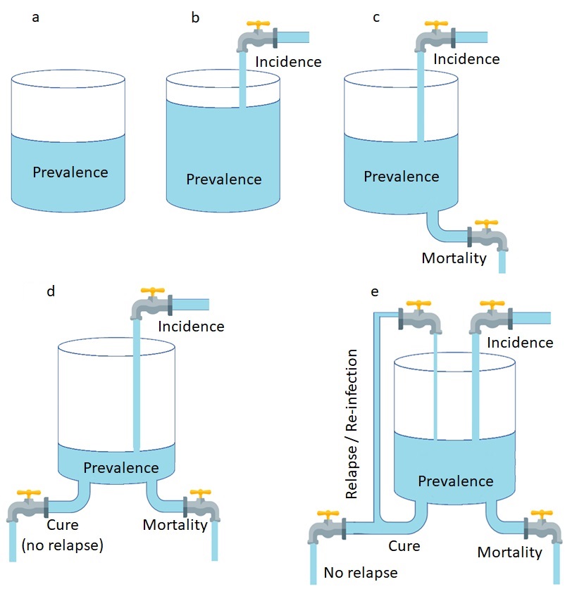
2.3.1a. Existing cases in the population (prevalence); 2.3.1b. Incidence increases prevalence; 2.3.1c. Mortality reduces prevalence; 2.3.1d. Cure reduces prevalence; 2.3.1e. Relapse and re-infection increase prevalence.

(Source for tap icon: https://www.iconexperience.com/g_collection/icons/?icon=water_tap)

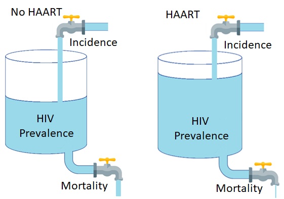
A real-world example of this relationship is the prevalence and incidence of HIV globally from 2000 to 2021. During this period, the incidence of HIV reduced from 2.9 million new cases per year in 2000 to just 1.5 million new cases per year in 2021. Meanwhile, the prevalence of HIV increased from 26.0 million people in 2000 to 38.4 million people in 2021 (Figure 2.3.2). During the same period, access to highly active anti-retroviral therapy increased from 2% in 2000 to 5% in 2005, 2.5% in 2010, 72% in 2020, and 75% in 2021 (World Bank, 2022). Although there is no cure for HIV, treatment with HAART greatly reduced HIV-related mortality, enabled people living with HIV to survive much longer, and increased the total prevalence of HIV in the process. Using the tank-and-flows analogy, HAART reduced the outflow of the water (mortality) while the inflow (incidence) continued; thus, the water in the tank (prevalence) increased (Figure 2.3.3).

Figure 2.3.2 Global prevalence and incidence of HIV from 2000 to 2021 (in millions of persons)

Source: UNAIDS, 2022

Figure 2.3.3 Analogy of how the increase in the use of highly active anti-retroviral therapy (HAART) affected the global prevalence of HIV

2.4 Limitations in Defining Numerators and Denominators of Incidence and Prevalence

Despite the relatively straightforward definitions of prevalence and incidence, as the number of cases and new cases divided by either the number of persons or person-time, the actual measurement of prevalence and incidence is complicated due to several existing limitations.

One group of limitations pertains to the numerators: counting the number of persons with the disease in a population (for prevalence) or new cases (for incidence) is complicated. For example, clinical depression is a common mental illness, with lifetime cumulative incidence ranging from 8% to 18% of the entire population in most countries (Kessler & Bromet, 2013). Diagnosis of clinical depression generally starts when a patient is assessed by a health worker with assessment tools. Assessment tools are not designed to diagnose but rather to measure the severity of depressive symptoms and refer individuals with more severe symptoms to a mental health specialist (i.e., a suitably trained general practitioner, psychiatrist, or psychologist). The mental health specialist then makes a detailed and holistic diagnosis assessment, which may include an assessment of the patient’s current mood and thought contents (e.g., hopelessness, pessimism, self-harm, suicide, and a lack of positive thoughts or plans). The specialist then generally follows guidelines set in the Diagnostic and Statistical Manual of Mental Disorders, Fifth Edition (DSM-5), which states that for the diagnosis of clinical depression, an individual must experience at least 5 of 9 specified symptoms during the same 2-week period, with one of the symptoms being either depressed mood or loss of interest or pleasure (Substance Abuse and Mental Health Services Administration., 2016).

To count the number of existing cases (numerator of prevalence) or the number of new cases (numerator of incidence) in a susceptible population, several issues must be considered as they may lead to inaccuracies:

Seeking initial assessment or care for mental health issues is stigmatized in many places worldwide; thus, not all persons who have clinical depression seek assessment and care for their depressive symptoms. This stigma and voluntary refusal of screening and treatment can make the reported prevalence lower than the true value. (See Chapter 11: Bias for more information.)

Screening is the process that determines whether a potential patient is referred to a mental health specialist; thus, the number of persons referred and diagnosed depends on the screening tool used. There is a large variety of screening tools, and the time period in some of these tools may not be 2 weeks like the DSM-5 criteria (American Psychological Association, 2022).

Screening programs may not be available at all primary health care providers, and in under-served areas, access to mental health specialists who can diagnose clinical depression may also be limited. Therefore, the number of persons screened and diagnosed depends on the availability of health services in each local area.

Another group of limitations pertains to the denominator: counting the number of susceptible (disease-free) persons in the population. In epidemiology, investigators must count either all the members of the population at the time of outcome measurement (for prevalence), the number of disease-free persons at the beginning of the follow-up period (for cumulative incidence), or the time that these persons spent in follow-up (for incidence rate or incidence density). The following limitations may occur when counting the denominator:

Denominators can be hard to define in populations that are marginalized, persecuted, or otherwise hidden. For example, if we are to assess the prevalence or incidence of clinical depression among people who inject drugs (PWIDs, formerly referred to as injection drug users or IDUs) using data from national surveys, it is likely that drug use is under-reported due to social desirability; therefore, the true denominator (total number of PWIDs in a population) is unknown, and the calculated prevalence or incidence is subject to uncertainty due to this unknown true denominator.

If we are to use data from a health facility, such as a psychiatric hospital, it is important to keep in mind that local patients may opt to receive care at another facility and that patients who come to the facility may be referred from places farther away. Defining the suitable denominator to enable the accurate estimation of incidence and prevalence of health outcomes may be difficult in this situation.

Most populations have incoming migration (immigration) and outgoing migration (emigration). Persons with clinical depression immigrate and emigrate; thus, the prevalence and incidence of depression also depend on the extent to which immigration and emigration occur at the time of measurement.

2.5 Critiquing the Measurement of an Exposure or an Outcome

In epidemiology, validity refers to the extent to which collected information reflects what one intends to measure, i.e., the accuracy of a given measurement. Despite the simple conceptualization of epidemiology as an exercise in counting the number of individuals in a population with particular attributes of interest, the actual practice in measurement is complex owing in part to issues regarding validity. Given that there is an overlap between psychology and epidemiology, the author wishes to summarize the following concepts in validity as described in a classical paper in psychology (Cronbach & Meehl, 1955), which describes four types of validity:

Predictive validity refers to the extent to which a criterion (an outcome) obtained after a test is given (or a question is asked) corresponds to the test or the question. For example, the GRE aptitude test is administered to applicants of nearly all graduate programs at universities in the United States. The questions on the test include an understanding of advanced English vocabulary and basic mathematics, primarily arithmetic and algebra. Although graduate-level education is more specialized and complex than these exams, the correlation between the scores and the graduate school performance of test-takers justifies the use of the scores by various programs as an assessment and potential prediction of the ability to succeed in graduate education; therefore, many graduate programs set minimum GRE scores for applicants.

Concurrent validity refers to the extent to which a criterion (outcome) obtained at the same time as the test (or the question) corresponds to the test or the question. For example, a test may correlate with a contemporary psychiatric diagnosis.

Content validity refers to the extent to which the test items (or questions) are a sample of a universe in which the investigator is interested. Content validity is assessed by deductively defining the universe (i.e., an exhaustive list) of test items or questions that can be administered and systematically sampling within this university to create the test or questions of interest.

Construct validity refers to the extent to which test items (or questions) can be interpreted as a measure of an attribute or quality that is not operationally defined. In psychology and social sciences, a construct refers to a conceptual idea or theory that is generally subjective. Unlike content validity, construct validity measures an attribute where “no criterion or universe of content is accepted as entirely adequate to define the quality to be measured” (Cronbach & Meehl, 1955). Examples of constructs include gender, race, self-esteem, and financial solvency. Assessment of construct validity is made when there is no way to directly measure a given variable; thus, an indirect measurement is required.

Considering construct validity is especially important in health sciences, particularly behavioral health, because constructs are complex. Physical attributes can be measured directly. It is possible and objective to count the number of teeth remaining in someone’s mouth. One cannot directly measure gender, race, self-esteem, or financial solvency. For example, in a study on the association between personal finances and health, there is a hypothesis that personal financial solvency is associated with the prevalence of anxiety. In personal finance, solvency refers to the “ability for one to pay their debts” (Billings, 2022). Based on this broad conceptualization, the range of questions to measure this construct seems infinite, and an investigator may opt to adopt the questions used by the U.S. Federal Reserve on the possible courses of action for participants to pay for a small financial emergency or to support themself for a particular period of time as a proxy measure of personal financial solvency with the question: “Suppose that you have an emergency expense that costs 5,000 Bahts. How would you find money to pay for this expense within a week?” (Wichaidit et al., 2022).

When one provides critiques of measurements in epidemiology, such as when writing a discussion section in a manuscript or conducting a journal club session, it is useful to refer to this notion of the potential discrepancies between what questions are asked (or what observations are made) by investigators, compared to the health outcomes or exposures that are being measured. For example, there are two main issues with the above-mentioned measurement of personal financial solvency. Firstly, the question refers to a hypothetical scenario (“Suppose that…How would you…”) with no details regarding the other circumstances that determine one’s actions. The response to this question is hypothetical by default and may not correspond to the real-world course of action that one would take. Secondly, the ability to pay debts may also vary depending on the amount of debt in question and the circumstances in which the debt needs to be paid. Thus, the answer only provides a sliver of the broader construct of solvency in personal finance. After extensive contemplation, one then finds a way to succinctly communicate one’s ideas and further contemplate better ways to improve the accuracy of the construct in future studies. If an investigator is able to continue conducting research on the same topic, it is advisable to re-read one’s own discussion remarks as well as recent literature on the construct of interest and consult with colleagues and experts on how to make measurements that are more valid in subsequent studies.

2.6 Practical Exercise: Calculation of Prevalence of Outcome and Exposure from Survey Data using R

To practice calculating the prevalence of outcome and exposure from survey data, please consider the following article published in PeerJ:

Wichaidit, W., Prommanee, C., Choocham, S., Chotipanvithayakul, R., & Assanangkornchai, S. (2022). Modification of the association between experience of economic distress during the COVID-19 pandemic and behavioral health outcomes by availability of emergency cash reserves: Findings from a nationally-representative survey in Thailand. PeerJ, 10, e13307. https://peerj.com/articles/13307/

In this article, we assessed the extent to which experience of economic distress during the COVID-19 pandemic affected behavioral health outcomes (including anxiety and depression). Investigators also assessed the extent to which the availability of an emergency cash reserve modified this association. For our exercise, we will simplify the analysis. The availability of a cash reserve will be our EXPOSURE, while the period prevalence of anxiety will be our OUTCOME. In this chapter, we will not yet assess the extent to which the EXPOSURE is associated with the OUTCOME, but instead, we will simply describe the distribution of the EXPOSURE, OUTCOME, and other characteristics of the study population separately in a table titled “General characteristics of the study population”.

The manuscript, data source, data dictionary, and study questionnaire can be accessed using the links in the following table:

Material	QR code	URL
Manuscript		https://peerj.com/articles/13307/
Data set		https://dfzljdn9uc3pi.cloudfront.net/ 2022/13307/1/ Suppl_-_Data_for_PeerJ.csv
Data dictionary		https://dfzljdn9uc3pi.cloudfront.net/ 2022/13307/1/ Suppl_-_Data_Dictionary_20210625.csv
Questionnaire		https://dfzljdn9uc3pi.cloudfront.net/ 2022/13307/1/ Questionnaire_TH_EN_20210624.pdf

In short, the dataset used in this exercise comes from a phone-based interview survey with 1555 participants. The survey questions that gave rise to this dataset include those pertaining to alcohol consumption, experience of economic distress, management of emergency expenses, screening instruments for depression and anxiety, mental health outcomes, and common demographic and socioeconomic characteristics. All supplementary materials are available in the mentioned links. The data are anonymized, de-identified, and have undergone data cleaning.

 

First, we need to clearly define our variables of interest, particularly our outcome and exposure. Please consider the variable definitions in Table 2.6.1, as well as the skeletal table for the characteristics of the study population in Table 2.6.2.

 

Table 2.6.1 Variable definition and analysis plan to describe the extent to which the availability of an emergency cash reserve (EXPOSURE) is associated with period prevalence of anxiety (OUTCOME) in the general population of Thailand in 2021

Variable	Definition	Coding
Exposure: Availability of an emergency cash reserve at baseline	Variable Q11 contains the measurement questions. We considered participants who answered that they would cover the emergency expense “With the money in [their] savings account, cash, or other liquid assets (e.g., converting mutual funds to cash)” without also answering that they would use their credit card, take out loans or lines of credits, or sell/pawn personal possessions to be those with available emergency cash reserves.	cash <- q11_3 shortcredit <- q11_1 longcredit <- q11_2 loanbank <- q11_4 borrow <- q11_5 loanshark <- q11_6 sell <- q11_7 pawn <- q11_8 cannot <- q11_9 others <- shortcredit + longcredit + loanbank + borrow + loanshark + sell + pawn + cannot cashonly <- ifelse(cash==1 & others==0, 1, 0)
	Those who indicated that they refuse to answer the question will be treated as having missing data.	refuse_answer <- q11_99 cashonly <- ifelse(refuse_answer==1, NA,cashonly)
Outcome: Prevalence of anxiety disorder	Variables q13gad_1 thru q13gad_7 contain the measurement questions GAD-7 score from the sum of questions 1 through 7 in section 13 (the GAD-7 section). Each score ranged from 0 to 3, so the total range = 0 to 21.	gad7_score <- q13gad_1 + q13gad_2 + q13gad_3 + q13gad_4 + q13gad_5 + q13gad_6 + q13gad_7
	If GAD-7 score is >= 10, then the respondent would be considered to have an anxiety disorder—otherwise, no anxiety disorder.	anxiety <- ifelse(gad7_score>=10, 1, 0)
Characteristics of study participants
Gender	Birth gender of the study participant, presented as appeared in the questionnaire; exclude those who refused to answer (missing values).	variable ‘sex’
Age	Age of the participants in year, assumed to be normally distributed; exclude those who refused to answer (missing values).	variable ‘age’
Marital status	Marital status of the study participants, presented as appeared in the questionnaire; exclude those who refused to answer.	variable ‘status’
Highest level of education completed	Highest level of education the study participants reported to have completed.	variable ‘edu’
	Matthayom 3 or less merged into the same category of “Junior High School or less”.	edu_recat <- ifelse(edu>=1 & edu<=3, “1 – Junior HS or less”, “Unknown”)
	Matthayom 6 and PorWorChor merged into the same category of “High school or equivalent”.	edu_recat <- ifelse(edu==4 | edu==5, “2 – High school or equivalent”, edu_recat)
	PorWorSor and Associate’s Degree merged into the same category of “Associate’s Degree or equivalent”.	edu_recat <- ifelse(edu==6 | edu==7, “3 – Assoc or equivalent”, edu_recat)
	Other categories are as they appeared in the survey (“Bachelor’s degree”) and (“Graduate degree”).	edu_recat <- ifelse(edu==8, “4 – Bachelor’s degree”, edu_recat) edu_recat <- ifelse(edu==9, “5 – Graduate degree”, edu_recat)
	Exclude those who refused to answer.	edu_recat <- ifelse(edu==999, NA, edu_recat) tab1(edu_recat)
Personal monthly income	Personal monthly income of the study participants	variable ‘salary’
	Exclude those who refused to answer.	salary_recat <- ifelse(salary==999,NA,salary)
	Otherwise presented as appeared in the questionnaire.	tab1(salary_recat)

Adapted from Wichaidit et al., 2022

Table 2.6.2 Draft (shell) table for the general characteristics of the study participants

Characteristic	Baseline (n = …)
Gender
Male
Female
Age (years) (mean ± SD)
Marital Status
Single
Married with child(ren)
Married, no children
Widowed/divorced /separated
Highest Level of Education Completed
Junior high school or lower
High school or equivalent
Associate’s degree or equivalent
Bachelor’s degree
Graduate degree
Personal Monthly Income
No more than 5,000 THB
5,001–10,000 THB
10,001–20,000 THB
20,001–30,000 THB
30,001–40,000 THB
40,001–50,000 THB
More than 50,000 THB
Emergency Expense: Suppose that you have an emergency expense that costs 5,000 THB, how would you pay for this expense within one week? (multiple responses allowed)
Put it on my credit card and pay it off in full on the next statement.
Put it on my credit card and pay it off in installments.
With the money in my savings account, cash, or other liquid assets
Using money from a bank loan or line of credit
Borrowing from friends or family members
Using a payday loan, deposit advance, or overdraft
Selling a personal belonging
Pawning a personal belonging
I would not be able to find money to pay for the expense.
Participants with 5000 THB in emergency cash reserves available
Anxiety disorder according to the GAD-7 questionnaire
No anxiety (GAD-7 < 10 points)
Anxiety (GAD-7 ≥ 10 points)

Our R codes for the analysis generally follow the “Coding” column in the variable definition and analysis plan, and we fill in the data results table accordingly (Table 2.6.3).

Table 2.6.3 General characteristics of the study participants

Characteristic	Frequency (%)
Gender
Male	751 (48.3%)
Female	804 (51.7%)
Age (years) (mean ± SD)	41.3 ± 12.9
Marital Status
Single	473 (30.4%)
Married with child(ren)	930 (59.8%)
Married, no children	70 (4.5%)
Widowed/divorced/separated	82 (5.3%)
Highest Level of Education Completed	(n = 1553)
Junior high school or lower	574 (37.0%)
High school or equivalent	430 (27.7%)
Associate’s degree or equivalent	153 (9.9%)
Bachelor’s degree	371 (23.9%)
Graduate degree	25 (1.6%)
Personal Monthly Income
No more than 5,000 THB
5,001–10,000 THB
10,001–20,000 THB
20,001–30,000 THB
30,001–40,000 THB
40,001–50,000 THB
More than 50,000 THB
Emergency Expense: Suppose that you have an emergency expense that costs 5,000 THB, how would you pay for this expense within one week? (multiple responses allowed)
Put it on my credit card and pay it off in full on the next statement.
Put it on my credit card and pay it off in installments.
With the money in my savings account, cash, or other liquid assets
Using money from a bank loan or line of credit
Borrowing from friends or family members
Using a payday loan, deposit advance, or overdraft
Selling a personal belonging
Pawning a personal belonging
I would not be able to find money to pay for the expense.
Participants with 5000 THB in emergency cash reserves available (n=1510)
Anxiety disorder according to the GAD-7 questionnaire
No anxiety (GAD-7 < 10 points)
Anxiety (GAD-7 ≥ 10 points)

Readers are encouraged to fill in the rest of the table by themselves. Solutions to this exercise can be found at the end of this chapter.

2.7 Conclusion

In this chapter, we covered the definition of prevalence (the number of existing cases in a population divided by the population size), which can be further classified as point prevalence (where the numerator is the number of existing cases at the time of measurement) and period prevalence (where the numerator is the number of existing cases during a given period of time). We also covered the definition of incidence (the number of new cases in a population divided by the number of susceptible persons or person-time in the population of interest during the observation period), which can be further classified as cumulative incidence (where the numerator is the number of susceptible persons) and incidence rate or incidence density (where the numerator is the total amount of time observed among susceptible persons, called “person-time”). Additionally, we covered the relationship between prevalence, incidence, and time with the formula Prevalence ≈ Incidence × Average duration. Lastly, we covered the limitations in measuring incidence and prevalence, as well as a brief overview of validity and how to apply concepts pertaining to validity to the critique of epidemiological measurement.

The author hopes that the exercise at the end of this chapter serves as a practical guide in statistical computing for interested readers.

References

American Psychological Association. (2022). Depression Assessment Instruments. https://www.apa.org/depression-guideline/assessment

Billings, J. (2022). What is Solvency? Personal Finance Lab. https://www.personalfinancelab.com/finance-knowledge/finance/what-is-solvency/

Cronbach, L. J., & Meehl, P. E. (1955). Construct Validity in Psychological Tests. Psychological Bulletin, 52, 281–302.

Gordis, L. (2014). Epidemiology (5th edition). Elsevier Saunders.

Kessler, R. C., & Bromet, E. J. (2013). The epidemiology of depression across cultures. Annual Review of Public Health, 34, 119–138. https://doi.org/10.1146/annurev-publhealth-031912-114409

Substance Abuse and Mental Health Services Administration. (2016). DSM-5 Changes: Implications for Child Serious Emotional Disturbance. Substance Abuse and Mental Health Services Administration (US). https://www.ncbi.nlm.nih.gov/books/NBK519712/table/ch3.t5/

UNAIDS. (2022). Fact Sheet 2022. https://www.unaids.org/sites/default/files/media_asset/UNAIDS_FactSheet_en.pdf

US Center for Disease Control. (2014, July 2). Principles of Epidemiology: Glossary. https://www.cdc.gov/csels/dsepd/ss1978/glossary.html

Wichaidit, W., Prommanee, C., Choocham, S., Chotipanvithayakul, R., & Assanangkornchai, S. (2022). Modification of the association between experience of economic distress during the COVID-19 pandemic and behavioral health outcomes by availability of emergency cash reserves: Findings from a nationally-representative survey in Thailand. PeerJ, 10, e13307. https://doi.org/10.7717/peerj.13307

World Bank. (2022). Antiretroviral therapy coverage (% of people living with HIV). https://data.worldbank.org/indicator/SH.HIV.ARTC.ZS