Chapter 1: What is Epidemiology?

Wit Wichaidit

1 Chapter 1: What is Epidemiology?

Objectives

After completing this module, you should be able to:

Define epidemiology and list the assumptions of epidemiology.

Define the determinants of disease.

Describe the concepts of investigating disease distribution by person, place, and time.

Describe the relationship between epidemiology and public health.

Describe the history of epidemiology.

Set up your computer for data analysis.

1.1 Introduction

Epidemiology is the study of the distribution of diseases and their determinants, and the application of this study to control health problems. Epidemiology is based on three fundamental assumptions (LaMorte, 2017):

1. Diseases do not occur at random. For any disease, there are determinants (causal or preventive factors) that can increase or decrease its likelihood of occurrence.

2. Determinants of disease can be identified through the systematic investigation of the person, place, and time in/at which the disease occurs.

3. Knowledge of the association between diseases and their determinants can be applied to disease prevention and control.

As epidemiology also includes behaviors that can negatively affect health, the author wishes to extend the definition and assumptions of epidemiology to include health-related behaviors as well and refer to these entities as “health outcomes”. The term “health outcome” should be considered interchangeable with “disease” throughout this textbook.

1.2 Determinants of Disease

A “determinant” generally refers to any factor that influences health: biological, chemical, physical, social, cultural, economic, genetic, and behavioral (Bonita et al., 2006). Determinants generally include the causes (including biological, chemical, or physical agents), risk factors (including exposure to sources of agent), modes of transmission (CDC, 2012), and social and economic environments that influence the occurrence of health outcomes. However, the term “determinant” does not include public health actions taken after gaining knowledge of the association between influencing factors and health outcomes.

1.3 Distribution of Disease in Terms of Person, Place, and Time

An example of the investigation of person, place, and time of a health outcome can be found in the study of obesity — arbitrarily defined as having a body mass index (BMI) of higher than 30 kg/sq.m.

Person: Who?

Assessment of variation in the occurrence of a health outcome by personal characteristics can offer two types of insight: 1) insights on population sub-groups that are particularly burdened by the health outcome, which informs prioritization of resources; and 2) insights on potential determinants of disease, which informs future efforts in disease prevention and control. Common personal characteristics include, but are not limited to, the following attributes: age, sex, ethnicity, level of education, income, and occupation. Assessment of variation in disease prevalence (number or proportion of those with a health outcome of interest in the population) often involves categorization in order to ease the process. For example, in the description of the prevalence of obesity in the United States (Hales et al., 2020), age (years) was categorized as age groups (Figure 1.3.1).

Figure 1.3.1 Variation in prevalence of obesity in the United States by sex, age group, and race

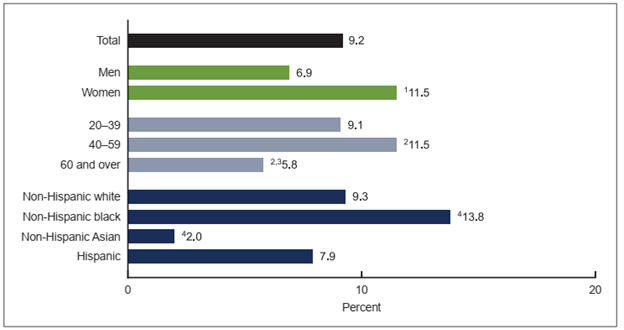
Source: Hales et al., 2020

Remarks:

¹Significantly different from men

²Significantly different from adults aged 20–39 years

³Significantly different from adults aged 40–59 years

⁴ Significantly different from all other race and Hispanic-origin groups

Based on the image above, obesity in the United States was more common (i.e., more prevalent) among women, those aged 40–59 years, and non-Hispanic Black people. Health programs to prevent and control obesity should prioritize these population groups accordingly. Furthermore, although it is not possible to infer the causes of obesity based on these findings, the findings nonetheless offer insights. Obesity is associated with health behaviors (Bookwalter et al., 2019), and assuming that people in different sub-groups behave differently, additional investigations into the health behaviors of these sub-groups may offer further insights into the determinants of obesity, which, in turn, may inform the design of new intervention programs to prevent and control obesity.

Place: Where?

Similar to the variation in the occurrence of a health outcome by personal characteristics, assessment of variation in health outcome occurrence by place (geographic distribution) can offer two types of insight: 1) insights on the geographic region particularly affected by the health outcome; and 2) insights on potential determinants of disease, which similarly informs future efforts in disease prevention and control (Figure 1.3.2).

Figure 1.3.2 Prevalence of adults who are overweight or obese by country (2016)

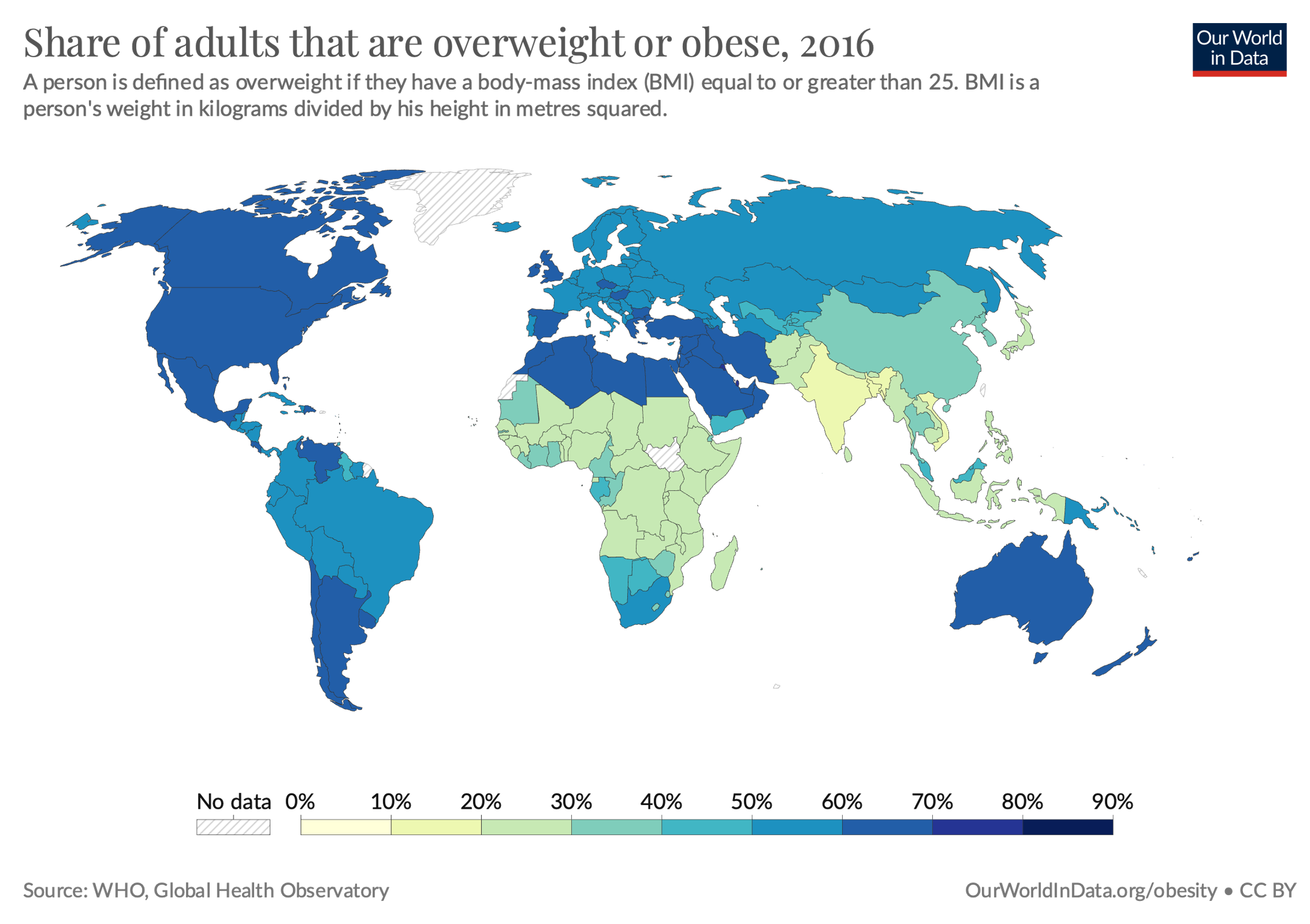
Source: Ritchie & Roser, 2017, https://ourworldindata.org/obesity#what-share-of-adults-are-obese

Obesity seems to be particularly high in the Americas, certain countries in Europe, North Africa and the Middle East, and Oceania. In that regard, determinants of health, such as socioeconomic conditions and health behaviors, tend to vary by geographic location. All of these factors affect the occurrence of obesity. Further investigations into the contexts and health behaviors of the local population in different countries and regions may similarly offer insights into risk factors and prevention strategies.

Time: When?

Assessing the variation in the occurrence of a health outcome by time can offer two types of insight: 1) insights regarding past and potential future trajectory (trend) of the outcome; and 2) insights regarding potential determinants of the outcome. However, it is important to be mindful that certain diseases, such as obesity, develop over years or decades. Thus, the time frame for presenting the trajectory or trend of such diseases should also be up to multiple decades (Figure 1.3.3).

Figure 1.3.3 Prevalence of adults who are overweight or obese in selected countries from 1975 to 2016

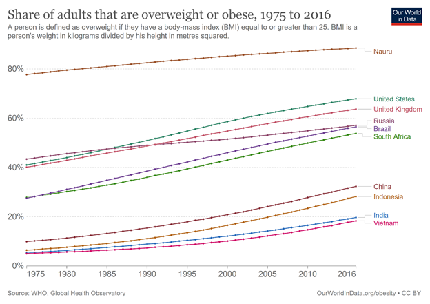
Source: Ritchie & Roser, 2017, Creative Commons BY license, https://ourworldindata.org/obesity#what-share-of-adults-are-obese

From the figure above, one trend is clear: the number of adults who are overweight and obese is rising in all countries. The slope of the line in each country offers insights into the magnitude of growth. From the figure, the increase appears to be more significant (with the line thus being steeper) in the emerging economies of China, Indonesia, India, and Vietnam, with Vietnam having the lowest obesity prevalence in the world. On the other hand, countries with historically high levels of overweight and obesity may now be at a point where the prevalence plateaus, as nearly the entire population has the outcome.

With regard to insights regarding potential determinants of the outcome, it is important to be mindful that determinants of health behaviors are dynamic. For example, during the COVID-19 pandemic, restrictions on alcohol purchase and consumption were enacted in order to limit alcohol-related social gatherings. Data on the prevalence of alcohol consumption during different policy periods may offer insights into the association between policy and alcohol consumption (Wichaidit et al., 2021) (Figure 1.3.4)

Figure 1.3.4 Summary of alcohol policy changes during the initial period of the COVID-19 pandemic in Thailand and the level of alcohol consumption (relative to the pre-pandemic level) after each change

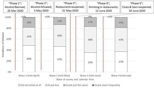
Source: Wichaidit et al., 2021

In the figure above, the white box can be considered as the proportion of the population who abstained from alcohol. The grey boxes, when merged, can be considered as the proportion of those who drank alcohol. There was a noticeable increase in the prevalence of alcohol consumption between Waves 2 and 3. This difference suggested that there was an association between the relaxation of on-premises drinking restrictions and alcohol consumption.

1.4 Controlling Health Problems: Epidemiology in Public Health, International Health, and Global Health

Epidemiology is classified by the US government as a sub-specialty in the sub-field of ecology, evolution, systematics, and population biology and is therefore classified as a STEM field (National Center for Education Statistics, 2020). Since epidemiology works with the population, there are three fields of study and action in which epidemiology is traditionally applied to control health problems at the population level: public health, international health, and global health. Although these three fields vary with regard to aims and foci (Table 1.4.1), these fields do overlap, and actions within one field (e.g., international health) may also be part of a broader set of actions in other fields (e.g., public health and global health). The differences highlighted within this text should thus be considered with a certain degree of flexibility in their interpretation.

Table 1.4.1 Public health vs. international health vs. global health, and the role of epidemiology

	Public health	International health	Global health
Aim	Preventing disease and promoting health	Providing health-related aid from industrialized countries to developing countries	Improving health and achieving equity in health for all people worldwide
Geographic focus	Particular community or country	Low and middle-income countries	N/A. Focus on issues that transcend national boundaries
Level of cooperation	Local	Bilateral (2 countries)	Global
Actions	Disease prevention in populations	Clinical care of individuals and disease prevention in populations	Clinical care of individuals and disease prevention in populations
Range of disciplines	Multidisciplinary (health sciences and social sciences)	Low level of multi-disciplinarity	Highly multidisciplinary (health sciences; social sciences; pure and applied science and mathematics; engineering and technology; humanities)
Roles of epidemiology	Public health surveillance; field investigation; analytic studies; evaluation; linkages/coordination; policy development	Public health surveillance; field investigation; analytic studies; evaluation; linkages/coordination; policy development	Public health surveillance; field investigation; analytic studies; evaluation; linkages/coordination; policy development

Adapted from CDC Division of Scientific Education and Professional Development, 2012; Douglas & Stemerding, 2013; Koplan et al., 2009; White & Nanan, 2008

To clarify, the roles of epidemiology in these fields of health refer to the following (CDC Division of Scientific Education and Professional Development, 2012):

Public health surveillance: To conduct a continuous and systemic “collection, analysis, interpretation, and dissemination of health data to help guide public health decision making and action” (CDC Division of Scientific Education and Professional Development, 2012).

Field investigation: To collect additional data to confirm or clarify the circumstances of reported information, identify additional cases, or identify the source(s) of illness, or to learn more about the disease of interest.

Analytic studies: To identify causes, mode of transmission, and appropriate control and prevention measures of a disease.

Evaluation: To systematically assess the effectiveness, efficiency, and impact of population health activities (e.g., disease control and prevention measures).

Policy development: To provide “input, testimony, and recommendations regarding disease control strategies, reportable disease regulations, and health-care policy” (CDC Division of Scientific Education and Professional Development, 2012)

1.5 History of Epidemiology

Although the term “epidemiology“ itself is fairly new, humans have likely practiced descriptive epidemiology, i.e., describing the distribution of health outcomes at the population level since the pre-historic period. This task would most likely have been performed by either the physician (“medicine man/woman”), the community leader (“tribal chief”), or the religious leader (“village shaman/shawoman”). Early data collection was likely based on observations and anecdotes, recorded by oral traditions. Remnants of past disease outbreaks and epidemics were in tales of terrible “plagues”. After the invention of writing, these plague tales became written records, and data collection became more systematic with the development of mathematics and natural philosophy. The author has summarized the major reported developments in epidemiology in the following table (Table 1.5.1).

Table 1.5.1 Timeline of epidemiology (extremely abridged, non-exhaustive)

Time	Event	Picture
c. 1600 BCE	A medical text written in Egyptian cursive hieroglyphs is authored. The majority of the manuscript describes 48 cases of trauma and surgery with a rational and scientific approach, which could be considered the first case series document in history. However, the text was likely a copy of an ancient text from the Old Kingdom period. American archaeologist James Henry Breasted speculated that the original author was *Imhotep* (27th century BCE). Today, the text is known as the Edwin Smith Papyrus.	Medical text written in Egyptian cursive hieroglyphs. Source: Jeff Dahl via Wikimedia Commons
c. 1350 BCE	Plague of Megiddo. Biridiya, mayor of Megiddo in ancient Canaan, sent a letter in clay tablet to the Pharoah of Egypt (likely Amenophis III). Biridiya reported that Megiddo was under threat from an invading army and that the city was being “destroyed by death as a result of pestilence and disease”. This was the first record of an epidemic, written in Akkadian cuneiform script. (DeeperStudy, 2024; Hanson, 2004; Wikipedia contributors, 2024). In other words, the tablet was the world’s first epidemiological report and the precursor to today’s MMWR.	Amarna Letter. Source: https://www.deeperstudy.com/link/amarna_letter.html
7th century BCE	The Book of Leviticus (13:45–46) describes procedures that individuals affected by the skin condition “tzaraath” must follow, including living away from the camps of the Israelites. The practice is the precursor to today’s quarantine.	Book of Leviticus (13:45–46) in Hebrew. Source: https://www.sefaria.org/Leviticus.13.45-46
c. 400 BCE	Hippocrates, the father of medicine, wrote De morbis popularibus (“Of the Epidemics“) and presented a thesis on environmental and behavioral causes of disease. He also wrote De aere, aquis et locis (“Of Air, Waters and Places”), describing the seasonality of diseases and the need for a good physician “to tell what epidemic diseases will attack the city, either in summer or in winter, and what each individual will be in danger of experiencing from the change of regimen,” essentially introducing the concept of endemicity and variations in person, place, and time of disease occurrence.	Source: Drawing of Hippocrates. https://blogs.acu.edu/ 1410_PSYC49301/2013/ 09/06/hippocrates-overcoming-the-fall/
168	Aelius Galenus (also known as Galen), described the Antonine Plague of 165–180. Galen produced a written description of the epidemic in a work titled Methodus Medendi (“Method of Treatment”), and he included the incidence, duration of disease, and prognosis of the cases. Estimated fatalities ranged from 2% to 33% of the Roman Empire, or 1.5 million to 25 million people. Today, scholars believe that the plague was caused by smallpox.	Painting depicting the Antonine Plague. Source: https://imperiumromanum.pl/ en/article/antonine-plague/
541	Justinian Plague. Procopius of Caesarea, a Greek scholar, reported on an epidemic of Yersinia pestis bubonic plague in the port of Pelusium, near Suez in Roman Egypt. The plague eventually spread throughout the Mediterranean Basin, Europe, and the Near East, killing between 25% to 60% of Europe’s population. The plague was likely the first pandemic in history. Procopius observed that Emperor Justinian’s court did not know how the disease spread and that religious rituals organized as a last resort were ineffective. Procopius thus evaluated, in this anecdote, the effectiveness of Rome’s intervention (religious ritual) by comparing the prevalence of the disease between the post-intervention (exposed) and pre-intervention (non-exposed) periods.	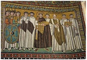A 6th century CE mosaic that shows Emperor Justinian and his court in the Basilica of San Vitale, Ravenna. Source: Carole Raddato (CC BY-SA)
1025	Persian polymath-physician-philosopher Ibn Sina (Latin: Avicenna) (980–1037) completed his most influential work, Qanun-e dâr Tâb قانون در طب (“The Canon of Medicine”). The Canon consisted of five books. Book 2 contained rules for experimenting with new drugs, which resembled the principles of clinical trials and causal inference. Book 5 contained cautions on possible stronger-than-expected effects when drug components were used together as compounds—a concept known today as interaction or effect modification.	Ibn Sina. Source: https://www.middleeasteye.net/discover/ibn-sina-who-persian-philosopher-physician-and-scientist
13th century	Muslim-Arab physician Ibn An-Nafis (1210–1288) commented on the translated version of De morbis popularibus in Sharh Kitab Al-Epidemic (“A commentary on Hippocrates’ Of the epidemics”), with arguments that people of different ages and genders had different biological processes and occupational hazards, introducing the concepts of confounding. He also provided a more detailed categorization of the seasons (exposures) and respiratory illnesses (outcomes). Additionally, Ibn An-Nafis described the location of malnutrition cases in Damascus with details that were sufficient for accurate mapping.	Source: https://muslimheritage.com/ibn-al-nafis-and-vinegar/
1346–1353	The second bubonic plague pandemic began with the Black Death, the most fatal pandemic recorded in human history. Physicians known as plague doctors were contracted by cities to treat infected patients. The doctors visited patients in their homes and recorded the number of dead and infected patients, essentially conducting public health surveillance.	A plague doctor. Paul Fürst, Der Doctor Schnabel von Rom. Source: Paul Fürst, Der Doctor Schnabel von Rom
1546	Italian physician Girolamo Fracastoro (1478–1553) published an essay titled Contagione et Contagiosis Morbis (“On Contagion and Contagious Diseases”). Fracastoro proposed that epidemic diseases were transferable by tiny particles or “spores” (chemical or living entities) that transmit infection by direct and indirect contact over long distances. He also introduced the concept of fomites, non-corrupted objects such as cloth and linen that can serve as a vessel of contagion. These ideas are the precursors to germ theory.	H.F. de sympathia et antipathia rerum liber unus. De contagione et contagiosis morbis et curatione libri III. Source: https://www.jnorman.com/pages/books/45020/girolamo-fracastoro/de-sympathia-et-antipathia-rerum-liber-unus-de-contagione-et-contagiosis-morbis-et-curatione
1598	Spanish physician Quinto Tiberio Angelerio (1532–1617) published a booklet describing his experience in the prevention and control of the 1582–83 plague in Sardinia, titled Epidemiologìa sive Tractatus de Peste (“Epidemiology or Treatise on Plague”). This was likely the first appearance of the word “epidemiology”.	Quincti Tyberii Angelerii Epidemiologia siue tractatus de peste. Source: https://www.europeana.eu/es/ item/9200110/Bibliographic Resource_1000126605974
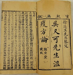
1641–1644	Chinese physician Wú Yòukě (吴又可) (1582–1652) observed various plagues and developed the idea that diseases were caused by transmissible agents called lì qì (戾气, “pestilential factors”). He published a 45-page treatise titled wēnyì fāng lùn (瘟疫方論, “Treatise on Pestilence”). Wu’s “pestilential factors” can be considered precursors to agents in germ theory.	Wú Yòukě’s writings. Source: https://www.seetao.com/details/16452.html
1665–1666	The Great Plague of London, the last major epidemic of the Second Pandemic, killed 100,000 Londoners (25% of the population). A tradesman, ward officer, and Royal Society member named *John Graunt* estimated the population of the City of London in order to assess the severity of the epidemic and observed the incompetence of the “searchers of the dead” in identifying the cause of death as being plague-related or otherwise, which could have introduced information bias to the assessment of disease-specific mortality. Graunt was perhaps the first epidemiologist.	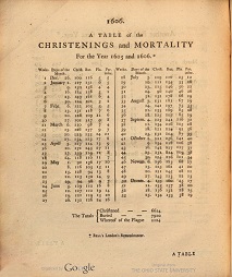Bill of Mortality for 1606. Source: The Collection of the Bills of Mortality from the archive from The Ohio State University via Wikimedia Commons
2–6 September 1666	A fire at a bakery in Pudding Lane started what became the Great Fire of London, burning much of the area with the City Wall. The plague stopped and did not recur.	Ludgate on fire. Source: Oil painting by an anonymous artist, c. 1670
1747	James Lind, a British Royal Navy surgeon on board the HMS Salisbury patrolling the Bay of Biscay off the coast of Spain, divided 12 sailors with similar symptoms of scurvy into 6 pairs. Each pair received the same diet and one unique remedy: 1) cider; 2) sulfuric acid; 3) vinegar; 4) seawater; 5) citrus fruits; 6) a mixture of spices. The pair on citrus fruits recovered within one week. Lind’s experiment was the first randomized clinical trial with six study arms.	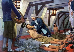Illustration of Lind caring for a sick patient aboard a ship. Source: Institute of Naval Medicine, https://www.bbc.com/ news/uk-england-37320399
1854	English physician John Snow used systematic data collection and dot mapping to describe the distribution of cholera cases during the 1854 Broad Street Cholera Outbreak and convinced local authorities that cholera was not caused by bad air (as per the miasma theory) but by contamination of the water from a pump on Broad Street. Authorities removed the force rod of the pump. The action is credited with ending the outbreak. Snow is considered as the founder of modern epidemiology.	Sample page from Snow’s On the mode of communication of cholera. Source: https://archive.org/details/ b28985266/page/138/ mode/2up?view=theater
1858	Florence Nightingale, the founder of modern nursing and pioneer in health management, published a manuscript on the causes of death among British soldiers on a campaign in Crimea. The quality of data visualization in her manuscripts continued to surpass others produced nearly two centuries later. Nightingale, F. (1858) Notes on Matters Affecting the Health, Efficiency, and Hospital Administration of the British Army. London: Harrison.	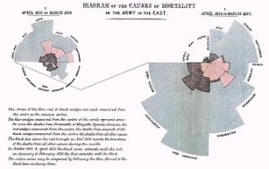Diagram of the Causes of Mortality in the Army in the East. Source: https://www.openculture.com/2016/03/florence-nightingale-created-revolutionary-visualizations-of-statistics-that-saved-lives-1855.html
1917	British physician Ronald Ross and mathematician Hilda Hudson published work on the application of mathematical theories on probability in epidemiology. The seminal paper included the susceptible-infectious-recovered (SIR) model, which described the transmission of infectious diseases from infective individuals to susceptible individuals and provided the basic framework for later epidemic models.	Dr. Ronald Ross, C.B. Source: https://collections.nlm.nih.gov/catalog/nlm:nlmuid-101427700-img Hilda Phoebe Hudson. Source: https://en.wikipedia.org/wiki/Hilda_Phoebe_Hudson#/ media/File:Hilda_Phoebe_Hudson.jpeg
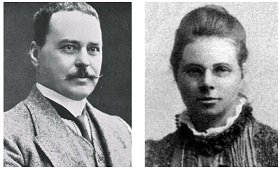
1950	Professor of Medical Statistics Austin Bradford Hill collaborated with British physician Richard Doll on a study examining the potential causes of lung cancer. The pair found that tobacco smoking was the only factor with consistent associations in all population groups. Doll then stopped smoking. Hill subsequently developed a group of nine principles for the assessment of causality, known as the Bradford Hill criteria.	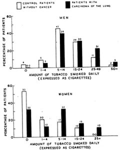Charts from Doll and Hill’s seminal work. Source: Doll & Hill, 1950
8 May 1980	The World Health Assembly of the World Health Organization declared smallpox to be eradicated. This was the first disease eradication in human history.	Dr. D. A. Henderson and members of the World Health Organization’s Smallpox Eradication Program, 1979. Source: https://www.who.int/news /item/13-12-2019-who-commemorates -the-40th-anniversary-of-smallpox-eradication
5 June 1981	The AIDS pandemic officially began. U.S. Centers for Disease Control and Prevention officials reported five unusual cases of pneumocystis pneumonia (PCP) in Los Angeles in the Morbidity and Morbidity Weekly Report (MMWR) newsletter. PCP was later found to be linked to HIV infection.	MMWR publication, 1981. Source: CDC, 1981
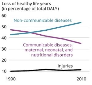
1990s	The burden of disease for non-communicable diseases surpassed infectious diseases combined with maternal and child health and nutritional problems worldwide. https://www.eea.europa.eu/data-and-maps/figures/the-shift-in-global-disease	Source: https://www.eea.europa.eu/data-and-maps/figures/the-shift-in-global-disease
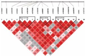
2005	Jonathan L. Haines and colleagues published a paper on the association between single-nucleotide polymorphism in the 1q32 chromosome and age-related macular degeneration (AMD), a landmark paper in genetic epidemiology and the first published genome-wide association study (GWAS).	Source: Haines et al., 2005
January 2020 to May 2023	The COVID-19 pandemic resulted in the death of 7 to 29 million people worldwide or 0.1–0.4% of the global population.	Atomic model of SARS-CoV-2. Source: https://en.wikipedia.org/wiki/COVID-19_pandemic#/media/File:Coronavirus._SARS-CoV-2.png
Mid-2020s	Here you are, reading this book.

1.6 Practical Exercise: Installing R and Setting Up Your Computer for Epidemiological Data Analysis

As mentioned in the Preface, this book is meant to serve as a practical guide for active learning of epidemiology. Despite what recent images in the news about the global COVID-19 pandemic and movies such as Contagion would have you believe, the majority of epidemiologists spend their career in front of a computer, designing studies and working with data. As such, your workstation needs to be set up with that purpose in mind. Data sets mentioned as examples throughout this book are from sources and studies that are limited in size and can be contained in a standard laptop (such as the one used by the author in 2022).

The world of big data is emerging at the time of writing this book. The author praises the work of those who are pioneering the application of big data to public health, including colleagues who work on the Genome-Wide Association Study (GWAS) and those who work on personalized/genomic medicine. Like-minded readers who wish to work with big data and write syntaxes to analyze data directly from a server may wish to consult other textbooks.

The primary program for analysis of data in this book is R. Without further ado, let’s get started.

Please download R by following the instructions from this website and follow the instructions on the screen: https://cran.r-project.org/

To achieve a more friendly user interface, readers may wish to also download RStudio by visiting this website and following the on-screen instructions: https://posit.co/download/rstudio-desktop/

Once RStudio installations are complete, the reader should be able to see the program with the following parts. Codes are to be entered in the “Source” screening and run by clicking “Run” on the upper right corner. Those who did not install RStudio will simply open the R console and type in the codes directly.

R codes and annotations throughout this book will be in grey highlights.

Installing R packages

R also has extension programs called packages, developed by users, to perform more complicated tasks. For exercises throughout this book, readers will need to follow the instructions below to download and install a package called epicalc needed to perform data analyses.

A book written by the author of epicalc with detailed instructions and exercises can be found here: https://medipe.psu.ac.th/epicalc/pdf/Epicalc_Bookv2.pdf

First, open up R, and then download the package. The instructions are on this webpage: https://medipe.psu.ac.th/epicalc/

Windows user are to run the following codes:

install.packages(c(“readxl”,”knitr”,”kableExtra”))

install.packages(“epicalc”, repos = “https://medipe.psu.ac.th/epicalc”)

Mac (OS X) and Linux users are to run the following codes:

install.packages(c(“readxl”,”knitr”,”kableExtra”))

install.packages(“epicalc”, repos = “https://medipe.psu.ac.th/epicalc”,type=”source”)

After running the codes, the user can open the epicalc package with thelibrary()command as per the following codes:

library(epicalc)

Basic R

Without data entry (or importation of data), R functions like a calculator that can perform statistical tests. Please run the following commands and observe the results:

1+1

5-3

2*5

100/5

2^3

sqrt(9)

27^(1/3)

The concatenation command c() can put numbers into the same group and do multiple calculations simultaneously.

c(1,2,3,4,5)*3

Annotations: When writing R codes, it is highly useful to add annotations in order to denote the analysis procedures. Annotations can be added directly to the codes by putting the hashtag (#) symbol in front of a line of texts. All texts in the same line after the # will not be read or run by R.

Assigning values: In R, number(s) and other types of variables can be placed inside an object with an arrow symbol, known as the “assignment operator” <-. It is also possible to check the type of object using the class() command. Try the following codes:

#Multiplying a group of numbers with a number

a <- c(1,2,3,4,5)

b <- 3

a*b

class(a)

class(b)

#Putting texts together into a string with a separator space ” “

text1 <- “Hello”

text2 <- “world”

paste(text1, text2, sep=” “)

class(text1)

class(text2)

Importing data into R

Note: the data set and supporting file(s) are available at this webpage: https://www.kaggle.com/wichaiditwit/datasets

We can also use R to open datasets and perform analyses in addition to entering data manually. In this practical exercise, we will use a dataset named “Ch1_data.csv“. It’s a comma-separated value (CSV) file that can be opened as a text file or in a spreadsheet. In this exercise, we will import the file into R.

Please download the dataset from Kaggle and save it to a folder that you can access. We can then set a working directory by specifying the location of that folder on your computer using setwd(“”) command, and putting the file location inside. For this example, I have saved the file to desktop. Please make sure to replace all forward slashes \ with the backslashes /

#First, open the epicalc package

library(epicalc)

#Second, set working directory with setwd()

#Please don’t forget to change the forward slashes (“\”) into backslashes (“/”)

#EXAMPLE:

#setwd(“C:\Users\Desktop”) #this is not good

setwd(“C:/Users/Desktop”) #this is good

#Open the file with the same “use” command. Don’t forget the last name of the file

use(“Ch1_data.csv”)

The first thing that we want to do is to explore the dataset. We can ask R to list the entire data set using the following command:

.data

The table is very long, so we can use the head(.data) command to shorten the display

> head(.data)

id male age current_drinker

1 1001 1 37 0

2 1002 1 27 0

3 1003 0 32 0

4 1004 1 42 1

5 1005 1 30 1

6 1006 1 41 1

We can also ask R to just show the name and description of the variables in the data set with the following command

des()

The outputs are as follow

> des()

No. of observations = 40

Variable Class Description

1 id integer

2 male integer

3 age integer

4 current_drinker integer

This data is from a hypothetical survey of 40 persons with 4 characteristics:

id = The unique ID of each person who participated in the study

male = Whether the person’s sex is male (value=1) vs. female (value=0)

age = The age in years of the study participants

current_drinker = Whether the person has consumed alcohol within the past 12 months (value=1) vs. not in the past 12 months or never drank (value=0).

We can add descriptions of the variables to the data set using the label.var() command. Inside the brackets, we will need to specify the variable name, then add a description of the variable in quotation marks (“”). The changes will then show on the description. For example:

> label.var(id, “Unique ID”)

> label.var(male, “Male (1) vs. Female (0) sex”)

> des()

No. of observations = 40

Variable Class Description

1 id integer Unique ID

2 male integer Male (1) vs. Female (0) sex

3 age integer

4 current_drinker integer

You can also create new variables by creating new objects based on the old one. For example, if you wish to create a new variable where someone who is male is labeled with the text “Male” instead of 0 in the variable ‘male’, you can create the new variable ‘male_text’ based on ‘male’. You can further specify the condition that if the value equals 1, the person is to be labeled “Male”, otherwise the person is labeled “Female”, as follows:

#Creating new variable

male_text <- ifelse(male==1, “Male”, “Female”)

However, after creating a new variable, the data set remains the same

head(.data)

des()

That is because we have not added the new variable to the dataset yes. This can be achieved using the label.var() command as follows:

label.var(male_text, “Sex of the participant in text file”)

head(.data)

des()

No. of observations = 40

Variable Class Description

1 id integer Unique ID

2 male integer Male (1) vs. Female (0) sex

3 age integer

4 current_drinker integer

5 male_text character Sex of the participant in text file

Exporting data from R

After you have worked on a dataset and created new variable, if you wish to export the data from R to the computer, you can use the command write.csv with the following template: write.csv(“filenamehere.csv”)

The new file will be saved at the same directory as the location you specified in the setwd() command. For example, if we were to name the updated dataset “Ch1_data_new.csv”, the command will be:

write.csv(.data, “Ch1_data_new.csv”)

Descriptive statistical analysis with R and the epicalc package

Univariate descriptive statistics

Now that we have covered how to import and export a dataset, let’s explore the dataset. First, we will look at how many participants are male and female.

We can obtain the frequency of the patients in each group with thetab1()command. Please note that the 1 after tab is the number one (1). For example:

> tab1(male)

male : Male (1) vs. Female (0) sex

Frequency Percent Cum. percent

0 12 30 30

1 28 70 100

Total 40 100 100

Now, please answer the following questions:

How many participants were in this data set?
How many participants (and how many percent of participants) were male?

We can do the same with the current drinking status

> tab1(current_drinker)

current_drinker :

Frequency Percent Cum. percent

0 21 52.5 52.5

1 19 47.5 100.0

Total 40 100.0 100.0

Now, please answer the following questions:

How many participants (and how many percent) were current drinkers?
How many participants (and how many percent) were not current drinkers?

Next, we can summarize the age of the participants using the command summary() or the command summ(), both of which would yield slightly different results:

> #Descriptive statistics for the participant’s age

> summary(age)

Min. 1st Qu. Median Mean 3rd Qu. Max.

19.00 28.00 33.00 37.67 49.00 66.00

> summ(age)

obs. mean median s.d. min. max.

40 37.675 33 13.039 19 66

Now, please answer the following questions:

What is the average (mean) age of the participants?
What are the minimum and maximum ages of the participants?

Bivariate descriptive statistics

In addition to the overall characteristics of the participants, we can gain more insights from the data by performing analyses with two variables at a time, a process known as bivariate analysis. One common procedure is to cross-tabulate the distribution of one variable with another. The R environment has the table() command that provides cross-tabulation without percentages, and the epicalc package has the tabpct() command that provides cross-tabulation with percentages. For example, if we wish to see the percent of men vs. women who are current drinkers, we can analyze the data as follows:

> table(male_text, current_drinker)

current_drinker

male_text 0 1

Female 6 6

Male 15 13

> tabpct(male_text, current_drinker)

Original table

current_drinker

Sex of the participant in text file 0 1 Total

Female 6 6 12

Male 15 13 28

Total 21 19 40

Row percent

current_drinker

Sex of the participant in text file 0 1 Total

Female 6 6 12

(50) (50) (100)

Male 15 13 28

(53.6) (46.4) (100)

Column percent

current_drinker

Sex of the participant in text file 0 % 1 %

Female 6 (28.6) 6 (31.6)

Male 15 (71.4) 13 (68.4)

Total 21 (100) 19 (100)

Please notice that the percentages are calculated by both rows and columns. In the example above in the outputs for tabpct(), the row percent showed the number and percentage of female participants with the current_drinkers values of 0 and 1 and the total, followed by the number and percentage of male participants with the current_drinkers values of 0 and 1 and the total. The column percent part showed the number and percentage of participants with current_drinker values of 0 who were female, male, and the total number, followed by the number and percentage of participants with current_drinker values of 1 who were female, male, and the total number.

Please answer the following questions:

What were the number and percentage of female participants who were current drinkers?
What were the number and percentage of male participants who were current drinkers?

We can also summarize numeric variables by group using the (“, by=”) option in the summ() command. For example, to compare the mean age between the male and female participants, we can use the following command:

> summ(age, by=male_text)

For male_text = Female

obs. mean median s.d. min. max.

12 34.583 28.5 15.986 19 64

For male_text = Male

obs. mean median s.d. min. max.

28 39 35.5 11.636 26 66

Please answer the following questions:

What was the mean age of the female participants?
What was the mean age of the male participants?

Answers to the exercise questions

ANSWER: 40 persons
ANSWER: 28 persons (70.0%)
ANSWER: 19 persons (47.5%)
ANSWER: 21 persons (52.5%)
ANSWER: 37.7 years
ANSWER: 19 years and 66 years, respectively
ANSWER: 6 persons (50.0%)
ANSWER: 13 persons (46.4%)
ANSWER: 34.6 years
ANSWER: 39.0 years

1.7 ConclusionEpidemiology is the study of the distribution of diseases (health outcomes) and their determinants, and then the application of this study to control health problems. Epidemiology is based on three assumptions: 1) diseases do not occur at random; 2) determinants of disease can be identified through investigation of the person, place, and time of occurrence; and 3) knowledge about the association between diseases and their determinants can be applied to disease prevention and control. Determinants include any factor that influences health. These factors can be identified by investing the persons in a population who were more and less likely to have the health outcome, the time in which the outcome occurs, and the places in which the outcome occurs. Humans have described the distribution of diseases since the first documentation of plague during the New Kingdom of Egypt, and these descriptions grew over time to include potential determinants of the plague. The description of this distribution became more detailed and includes the application of mathematics and other fields of science over time. Thank you for your interest in epidemiology.

ReferencesBonita, R., Beaglehole, R., & Kjellstrom, T. (2006). Basic Epidemiology (2nd ed.). WHO Press. http://whqlibdoc.who.int/publications/2006/9241547073_eng.pdf

Bookwalter, D. B., Porter, B., Jacobson, I. G., Kong, S. Y., Littman, A. J., Rull, R. P., & Boyko, E. J. (2019). Healthy behaviors and incidence of overweight and obesity in military veterans. Annals of Epidemiology, 39, 26–32.e1. https://doi.org/10.1016/j.annepidem.2019.09.001

CDC. (1981). Pneumocystis pneumonia—Los Angeles. MMWR. Morbidity and Mortality Weekly Report, 30(21), 250–252.

CDC. (2012, May 18). Lesson 1: Introduction to Epidemiology. Center for Disease Control and Prevention. https://archive.cdc.gov/#/details?url=https://www.cdc.gov/csels/dsepd/ss1978/lesson1/quizanswers.html

CDC Division of Scientific Education and Professional Development. (2012, May 18). Section 4: Core Epidemiologic Functions. Centers for Disease Control. https://www.cdc.gov/csels/dsepd/ss1978/lesson1/section4.html

DeeperStudy. (2024). Letter from Biridiya of Megiddo (EA 244). DeeperStudy. https://www.deeperstudy.com/link/amarna_letter.html

DOLL, R., & HILL, A. B. (1950). Smoking and carcinoma of the lung; preliminary report. British Medical Journal, 2(4682), 739–748. https://doi.org/10.1136/bmj.2.4682.739

Douglas, C. M. W., & Stemerding, D. (2013). Governing synthetic biology for global health through responsible research and innovation. Systems and Synthetic Biology, 7(3), 139–150. https://doi.org/10.1007/s11693-013-9119-1

Haines, J. L., Hauser, M. A., Schmidt, S., Scott, W. K., Olson, L. M., Gallins, P., Spencer, K. L., Kwan, S. Y., Noureddine, M., Gilbert, J. R., Schnetz-Boutaud, N., Agarwal, A., Postel, E. A., & Pericak-Vance, M. A. (2005). Complement Factor H Variant Increases the Risk of Age-Related Macular Degeneration. Science, 308(5720), 419–421. https://doi.org/10.1126/science.1110359

Hales, C. M., Carroll, M. D., Fryar, C. D., & Ogden, C. L. (2020). Prevalence of obesity and severe obesity among adults: United States, 2017–2018 (360; NCHS Data Brief). National Center for Health Statistics. https://www.cdc.gov/nchs/products/databriefs/db360.htm

Hanson, K. C. (2004, June 29). Amarna Tablet 244: Letter from Biridiya of Megiddo to Pharaoh. K. C. Hanson’s HomePage. https://www.kchanson.com/ANCDOCS/meso/amarna244.html

Koplan, J. P., Bond, T. C., Merson, M. H., Reddy, K. S., Rodriguez, M. H., Sewankambo, N. K., & Wasserheit, J. N. (2009). Towards a common definition of global health. Lancet (London, England), 373(9679), 1993–1995. https://doi.org/10.1016/S0140-6736(09)60332-9

LaMorte, W. W. (2017, October 18). What is Epidemiology? Boston University School of Public Health. https://sphweb.bumc.bu.edu/otlt/mph-modules/ep/ep713_history/EP713_History9.html

Ritchie, H., & Roser, M. (2017). Obesity. Our World in Data. https://ourworldindata.org/obesity

White, F., & Nanan, D. J. (2008). International and Global Health. In R. B. Wallace (Ed.), Maxcy-Rosenau-Last Public Health and Preventive Medicine (15th ed., pp. 1252–1258). McGraw Hill.

Wichaidit, W., Sittisombut, M., Assanangkornchai, S., & Vichitkunakorn, P. (2021). Self-reported drinking behaviors and observed violation of state-mandated social restriction and alcohol control measures during the COVID-19 pandemic: Findings from nationally-representative surveys in Thailand. Drug and Alcohol Dependence, 221, 108607. https://doi.org/10.1016/j.drugalcdep.2021.108607

Wikipedia contributors. (2024, October 2). List of epidemics and pandemics. Wikipedia, The Free Encyclopedia. https://en.wikipedia.org/w/index.php?title=List_of_epidemics_and_pandemics&oldid=1248917857

Media Attributions

Antonine_plague
Justinian
Ibn Sina
Ibn An Nafis
Plague_Doctor
Fracastoro
Angelerii
Wu_Youke
Bill_Mortality
London_Fire
James_Lind
John Snow
Nightingale
Ross_Hudson
Doll_Hill
WHO_Smallpox
MMWR
BoD
GWAS
COVID
Fig_1_7_1_RStudio

License

Icon for the Creative Commons Attribution-NonCommercial 4.0 International License

Epidemiology: An Introduction with a Focus on Behavioral Health Copyright © 2025 by Wit Wichaidit is licensed under a Creative Commons Attribution-NonCommercial 4.0 International License, except where otherwise noted.

Media Attributions

License

Share This Book