10 Chapter 10: Confounding
Chapter 10: Confounding
Objectives
After completing this module, you should be able to:
Describe the basic concepts in confounding.
Describe methods to control confounding.
Describe methods to identify potential confounders.
10.1 Introduction
When we consider findings in epidemiology, particularly those pertaining to the association between an exposure and an outcome, we should keep one question in mind: “Are these results real (reflecting the truth)? Or are they due to chance, bias, or confounding?” The answers to these questions provide us with alternative explanations for the observed findings that enable us to interpret data and the world around us in a more cautious manner.
10.2 Confounding in Epidemiological Studies
Confounding (from the Latin term “confundere”, “to mix together”) refers to a distortion of the association between an exposure and an outcome due to the presence of an extraneous variable in the study population. The extraneous variable (called the “confounder”) distorts the observed association from the true value because of a mixing of effects between it (the confounder) and the exposure of interest. This mixing of effects can make the measure of association (e.g., odds ratio, risk ratio) higher or lower than the true value.
Definition: “Confounding is the distortion of a measure of the effect of an exposure on an outcome due to the association of the exposure with other factors that influence the occurrence of the outcome” (Porta, 2008)
There are three requirements for a confounder:
The confounder must be associated with the outcome, independent of the exposure.
The confounder must be associated with the exposure.
The confounder must not be in the causal pathway between the exposure and the outcome.
A schematic representation of the concept of confounding can be found in Figure 10.2.1.
Figure 10.2.1 Conceptual diagram of the effect of a confounder on the association between an exposure and an outcome
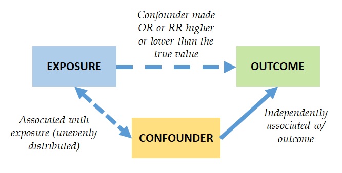
Adopted from Bonita et al., 2006
The association with the outcome independent of the exposure means that the confounder is an independent predictor or a determinant of the outcome. The confounder being associated with the exposure means that the confounder is unevenly distributed between exposed and non-exposed groups. The confounder not being in the causal pathway between the exposure and the outcome means that the confounder must not be an intermediate variable in the association between the exposure and the outcome. In other words, the confounder must not be something that is caused by the exposure, which then causes the outcome.
Consider the results of the following hypothetical cohort study with 2,000 persons. We want to investigate the association between coffee consumption and heart attacks. Our outcome of interest is having a heart attack (myocardial infarction) ten years after baseline data collection (had a heart attack vs. no heart attack). Our exposure of interest is coffee consumption (regular coffee drinkers vs. non-drinkers).
Table 10.2.1 Coffee consumption (at baseline) and heart attack (at one year follow-up) in a cohort study: possible confounding by smoking
|
|
|
Heart attack (Outcome) |
|
|
|
|
|
|
Yes (+) |
No (-) |
Total |
Incidence (Risk) of heart attack |
|
Coffee Drinking (Exposure) |
Regular coffee drinkers (Exposed) (+) (n = 1160) |
820 (a) |
340 (b) |
1160 (a+b) |
a/(a+b) = 820/1160 = 0.7068 = 70.68% |
|
|
Non-drinkers (Non-exposed) (-) (n = 840) |
180 (c) |
660 (d) |
840 (c+d) |
c/(c+d) = 180/840 = 0.2142 = 21.42% |
|
|
Total |
1000 |
1000 |
2000 |
|
Since cohort studies directly measure risk, we can calculate the unadjusted risk ratio (unadjusted RR) as follows:
Unadjusted Risk Ratio (Unadjusted RR):
Unadjusted RR = Incidence (among exposed) / Incidence (among non-exposed)
Unadjusted RR = 0.7068/0.2142 = 3.29 (95% CI = 2.99, 3.63)
Interpretation: Regular coffee drinkers had a 3.29 times higher risk (incidence) of having a heart attack compared to non-drinkers, and the difference is statistically significant.
Should we tell everyone to stop drinking coffee to reduce the risk of having a heart attack? Well, if we reached that conclusion without due diligence, many people in the coffee business would be angry at us forever. So, let us first think of alternative explanations. What other risk factors for heart attacks are there?
How about smoking? That is a viable alternative explanation. Smoking is a known determinant of heart disease regardless of whether someone drinks coffee or not (Requirement #1). People who drink coffee are more likely to be smokers than people who do not drink coffee (Requirement #2). Drinking coffee does not cause someone to smoke, i.e., smoking is not in the causal pathway between coffee consumption and heart attacks (Requirement #3).
Assessment of Requirement #1: Let us analyze data to test our hypothesis. Please consider the following table from the same cohort study data, comparing the incidence of heart attacks between smokers and non-smokers.
|
|
|
Heart attack (Outcome) |
|
|
|
|
|
|
Yes (+) |
No (-) |
Total |
Incidence (Risk) of heart attack |
|
Smoking |
Smokers (n = 1200) |
900 (a) |
300 (b) |
1200 (a+b) |
900/1200 = 0.7500 = 75.00% |
|
|
Non-smokers (n = 800) |
100 (c) |
700 (d) |
800 (c+d) |
100/800 = 0.1250 = 12.50% |
|
|
Total |
1000 |
1000 |
2000 |
|
Risk Ratio (RR) for smoking on heart attack:
RR = Incidence of heart attack among smokers / incidence of heart attack among non-smokers
RR = 0.7500/0.1250 = 6.00 (95% CI = 5.42, 6.64)
Smokers had a 6 times higher risk (incidence) of having a heart attack compared to non-smokers. Smoking met the first criterion for confounding: Smoking is significantly associated with the outcome (heart attack).
Assessment of Requirement #2: Let us now look a bit more deeply into the data. We will now compare smoking behaviors among coffee drinkers vs. people who do not drink coffee.
|
|
|
Smokers |
|
|
|
|
|
Yes |
No |
Total |
|
Coffee Drinking (Exposure) |
Regular coffee drinkers (Exposed) (n = 1160) |
1080 (93%) |
80 (7%) |
1160 (100%) |
|
|
Non-drinkers |
120 (14%) |
720 (86%) |
840 (100%) |
Nearly all (93%) coffee drinkers are smokers, but very few (14%) non-coffee drinkers are smokers. Smoking met the second criterion for confounding: Smoking is associated with the exposure (coffee drinking).
Assessment of Requirement #3: No data analysis for this part. We simply need to carefully consider the potential causality between coffee drinking, smoking, and heart attack. Smoking is a voluntary behavior. Coffee drinkers can decide not to smoke. So, we can say that drinking coffee does not have a causal relationship with smoking. Smoking met the third criteria for confounding: Smoking is not in the causal pathway between the exposure (coffee drinking) and the outcome (heart attack).
Smoking is an independent risk factor for heart attacks, and coffee drinkers are also smokers, so the effect of smoking could have been mixed with the effect of coffee drinking in the crude RR (3.92) that we calculated at the beginning. In this example, confounding by smoking distorts the observed measure of association (the crude RR) between coffee drinking (exposure) and heart attacks (outcome) from the true value.
10.2.1 Controlling for Confounding
Confounding distorts the observed association (crude RR) from the true value. We need to remove or reduce confounding in order to have a more valid (correct) estimate of the measure of association (adjusted RR). There are several ways to remove or reduce confounding: restriction, matching, randomization, and statistical adjustments (such as stratified analyses).
Restriction: We can restrict enrollment to only those subjects who have a specific value of the confounding variable. In our example, we can restrict the study to only include never smokers to remove the effect of smoking from the study.
Matching: Matching is the process of making a study group and a comparison group similar or identical with respect to their distribution of the confounder. We can match one comparison group to another on the confounder. In this example, we can match a coffee drinker who smokes to a non-coffee drinker who smokes, and we can also match a coffee drinker who does not smoke to a non-coffee drinker who does not smoke. Matching ensures comparability between the coffee drinkers and non-coffee drinkers groups with regard to smoking.
If we find a coffee drinker (exposed) person who smokes, we will find a non-coffee drinker who also smokes to join the comparison (non-exposed) group.
If we find a coffee drinker (exposed) who does not smoke, we will find a non-coffee drinker who also does not smoke to join the comparison (non-exposed) group.
Randomization: Random allocation (assignment or intentional giving) of the intervention (exposure) or control treatment (control) among the study participants. Randomization is done in randomized clinical trials and other experimental studies. Randomization of participants to exposed vs. non-exposed groups ensures equal distribution of the confounder between study groups; therefore, the effect of the uneven distribution of the confounder in the exposed and non-exposed groups could be substantially reduced.
Statistical adjustment: Using statistical techniques to control for confounding during data analysis. Such techniques can remove the effect of confounding from the measure of association (e.g., adjusted OR, adjusted RR). The adjusted estimates, in theory, will be closer to the true value.
A summary of the advantages and disadvantages of each method for controlling confounding can be found in the following table:
|
Method |
Advantages |
Disadvantages |
|
Restriction |
* Easy to understand * Focuses the sample of subjects for the research question
|
* May limit the number of eligible subjects * Residual confounding may persist if restriction categories are not sufficiently narrow * Limits generalizability: the conclusion of the study only applies to the population that was restricted for the study
|
|
Matching |
* Useful in preventing confounding that may be difficult to manage in any other way
|
* Finding appropriate matches may be difficult and expensive and limit sample size (may be hard to find a control with the same age, sex, AND smoking status as the comparison group) * In a case-control study, a factor used to match subjects cannot itself be evaluated as a risk factor for the disease
|
|
Randomization |
* Has the ability to control the effect of confounding for ALL variables, including the ones about which the investigator is unaware
|
* Applicable only for intervention studies (e.g., randomized trials) * Cannot always eliminate confounding
|
|
Statistical adjustment |
* Multivariable analysis makes it easy to control for two or more confounders at the same time. * Stratified analysis can be used to assess both confounding and effect modification (for more details, see the next section) |
* Cannot always eliminate residual confounding * Cannot always eliminate unmeasured confounding |
10.2.2 Stratified Analyses
One method to remove confounding by statistical adjustment is stratification. In the example, when we stratify, we are going to calculate two RRs instead of one. One RR will be the RR for coffee drinking and heart attacks only among smokers, and the other RR will be the RR for coffee drinking and heart attacks only among non-smokers.
The results of the stratified analyses are as follows:
|
|
|
Heart attack (Outcome) |
|
|
|
|
|
|
Yes (+) |
No (-) |
Total |
Incidence (Risk) of heart attack |
|
Among smokers only |
|
|
|
|
|
|
Coffee Drinking (Exposure) |
Regular coffee drinkers (Exposed) (+) (n = 1180) |
810 (a) |
270 (b) |
1080 (a+b) |
810/1080 = 0.75 = 75.00% |
|
|
Non-drinkers (Non-exposed) (-) (n = 120) |
90 (c) |
30 (d) |
120 (c+d) |
90/120 = 0.75 = 75.00% |
|
|
Total |
300 |
900 |
1200 |
Unadjusted RR = 0.75/0.75 = 1.00 |
|
Among non-smokers only |
|
|
|
|
|
|
Coffee Drinking (Exposure) |
Regular coffee drinkers (Exposed) (n = 1180) |
10 (a) |
70 (b) |
80 (a+b) |
10/80 = 0.125 = 12.50% |
|
|
Non-drinkers (Non-exposed) (n = 120) |
90 (c) |
630 (d) |
720 (c+d) |
90/720 = 0.125 = 12.50% |
|
|
Total |
700 |
100 |
800 |
Unadjusted RR = 0.125/0.125 = 1.00 |
Interpretation: Among smokers, regular coffee drinkers had the same risk (incidence) of heart attacks as non-coffee drinkers (RR = 1.00). There was no association between coffee drinking and heart attacks. Similarly, among non-smokers, regular coffee drinkers also had the same risk (incidence) of heart attacks as non-coffee drinkers (RR = 1.00). After controlling for the effect of smoking by stratification, there was no statistically significant association between coffee drinking and heart attacks.
Before stratification, study participants who drank coffee had a higher risk of having a heart attack than participants who did not drink coffee (crude RR = 3.29). However, stratified analyses showed that when stratified by smoking status, coffee drinkers had the same level of risk as non-coffee drinkers (RR among smokers = 1.00; RR among non-smokers = 1.00). Working with two stratified RRs is cumbersome, so there is a way to calculate a unified adjusted RR for the association between coffee drinking and heart attacks; this method is called the Mantel–Haenszel (MH) procedure.
10.2.3 Mantel–Haenszel (MH) procedure for adjusted analysis
If we want to combine the two stratified RRs into one adjusted RR to compare this to the crude RR. We can do so using the Mantel–Haenszel (MH) procedure, which is a statistical procedure for calculating a measure of association adjusted for a confounder (adjusted OR, adjusted RR, etc.) based on the assumption that the subjects in all tables were sampled from the populations with the same odds ratio.
The MH-adjusted RR in this example can be calculated as follows:
|
|
|
Heart attack (Outcome) |
|
|
|
|
|
Yes (+) |
No (-) |
Total |
|
Among smokers |
|
|
|
|
|
|
Regular coffee drinkers (Exposed) (+) (n = 1180) |
810 (a1) |
270 (b1) |
1080 (a1+b1) |
|
|
Non-drinkers (Non-exposed) (-) (n = 120) |
90 (c1) |
30 (d1) |
120 (c1+d1) |
|
|
|
|
|
Total = 1200 (n1) |
|
Among non-smokers |
|
|
|
|
|
|
Regular coffee drinkers (Exposed) (+) (n = 1180) |
10 (a2) |
70 (b2) |
80 (a2+b2) |
|
|
Non-drinkers (Non-exposed) (-) (n = 120) |
90 (c2) |
630 (d2) |
720 (c2+d2) |
|
|
|
|
|
Total = 800 (n2) |
In this example, the adjusted (pooled) MH estimates can be calculated using the following formula:
RRMH=∑ai(ci+di)/ni∑ci(ai+bi)/ni
In other studies in which odds ratios are calculated, the adjusted (pooled) MH odds ratio estimates can be calculated with the following formula:
ORMH=∑aidi/ni∑bici/ni
For example, in our study:
RRMH = {[a1(c1+d1)/n1] + [a2(c2+d2)/n2]} / {[c1(a1+b1)/n1] + [c2(a2+b2)/n2]}
RRMH = {[810*120/1200] + [10*720/800]} /{[90*1080/1200] + [90*80/800]}
RRMH = (27+63) / 27 + 63 = 90/90
RRMH = 1.00 (95% CI = 0.71, 1.40)
Interpretation: After adjusting for smoking using the Mantel–Haenszel procedure, coffee drinkers had the same risk of heart attacks as non-coffee drinkers.
Conclusion for Example 1: Before adjusting for confounders, coffee drinkers had a higher risk of having a heart attack than non-coffee drinkers (crude RR = 3.29). After adjusting for confounding by smoking, coffee drinkers had the same level of risk as non-coffee drinkers (M–H adjusted RR = 1.00). Smoking was a confounder in the association between coffee drinking and heart attacks. Coffee drinking was actually not associated with heart attacks (see Figure 10.1.2).
Figure 10.2.3.1 Conceptual diagram of the confounding of the association between coffee drinking and heart attacks by smoking
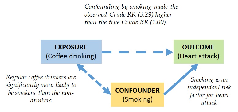
Adopted from Bonita et al., 2006
10.2.4 Multivariable Analyses
As an alternative to the Mantel–Haenszel procedure, and if you wish to adjust for multiple confounders at the same time, one commonly used technique to adjust for confounding during data analysis is to adjust for multiple variables at the same time. The procedures are beyond the scope of this course, and interested individuals should consult any book on statistical analysis in epidemiology and look under multivariable analyses.
10.3 Methods for Identification of Confounders
Confounding can be assessed using several methods: 1) Existing (a priori) understanding of the determinants of the disease of interest; 2) Assessment as per the requirements of the confounder; 3) Assessment based on stratified and adjusted analyses.
10.3.1 Existing (a priori) Understanding of the Determinants of the Disease of Interest
This is the author’s preferred method of identifying confounders. One of the author’s mentors taught the author that to be a good epidemiologist, one needs to be as knowledgeable as possible about the outcome of interest. With a solid foundation regarding the determinants of the outcome of interest, one may choose confounders to adjust and control based on the existing (a priori) understanding of the disease. In the author’s recent article on the association between cannabis outlet density and cannabis use behaviors (Wichaidit et al., 2024), the authors described the data analysis process as follows:
“For multivariate analyses, previous studies have found that cannabis use is associated with sex (Fond et al., 2021), tobacco smoking (Fond et al., 2021), marital status (El Marroun et al., 2008), religion (El Marroun et al., 2008), educational level (El Marroun et al., 2008). Meanwhile, cannabis use disorder is associated with sex (Fond et al., 2021), tobacco smoking (Fond et al., 2021), income (Mair et al., 2021), unemployment (Mair et al., 2021), and age of onset of cannabis use (Schlossarek et al., 2016). Thus, in multivariate analyses for our study outcomes, we adjusted for the participant’s sex, age, tobacco smoking status, marital status, income, religion, occupation, educational level, and age of onset of cannabis use as confounders based on a priori identification according to the literature.”
Source: Wichaidit et al., 2024
10.3.2 Assessment as per the Requirements of the Confounder
Some epidemiologists may choose to assess confounding by going through each of the confounder requirements as follows:
The confounder must be associated with the outcome independent of the exposure: This can be done simply by using bivariate analyses (cross-tabulation and logistic regression) of the extraneous variable vs. the outcome. If the association is significant, then the extraneous variable meets the first requirement of the confounder.
The confounder must be associated with the exposure: This can be assessed statistically by crosstabulating the distribution of the extraneous variable by the exposure. If the distribution of the extraneous variable significantly differed between the exposed vs. non-exposed groups, then it meets the second requirement of the confounder.
The confounder must not be in the causal pathway between the exposure and the outcome: The statistical process of identifying confounders generally ends at Requirement #2. Assessment of whether the confounder met Requirement #3 can be based on the knowledge (coming from the fields of biomedical or social sciences) of the potential causal pathway between the exposure and the outcome. If the exposure potentially causes the extraneous variable, which then causes the outcome, then the extraneous variable is a pathway variable and not a potential confounder.
10.3.3 Assessment Based on Stratified and Adjusted Analyses
Some epidemiologists may choose to stratify their analyses by levels of the confounder or adjust for the effect of the confounder in multivariable data analyses. As shown in the Stratified Analyses section earlier in this chapter on the association between coffee drinking and heart attacks:
|
Measure of association between coffee drinking (exposure) and heart attacks (outcome) |
RR |
|
Crude RR (all participants) |
RR_crude = 3.29 (95% CI = 2.99, 3.63) |
|
Stratified RR (association among smokers only) |
RR_smokers = 1.00 (95% CI = 0.72, 1.38) |
|
Stratified RR (association among non-smokers only) |
RR_non_smokers = 1.00 (95% CI = 0.92, 1.09) |
|
Mantel–Haenszel (MH) Adjusted RR (adjusted for smoking) |
RR_adjustedMH = 1.00 (95% CI = 0.71, 1.40) |
Generally, when the crude measure of association is higher (or lower) than ALL stratified measures of association, then the stratifying variable (in this case, smoking) is a potential confounder. Alternatively, if the following calculation for percentage change in the measure of association is 10% or more, the general guideline and practice in epidemiology is to consider the adjusting variable (in this case, smoking) to be a potential confounder:
Percentage_change = [(RR_crude – RR_adjusted) / RR_crude] * 100
In the example of the association between coffee drinking and heart attacks, the percentage change is:
Percentage_change = [(3.29 – 1.00) / 3.29] * 100 = 2.29/3.29 * 100 = 69.6%
Adjusting for smoking changed the RR in the association between coffee drinking and heart attacks by 69.6%—which is more than 10%! Therefore, smoking is a potential confounder.
The RR here can be substituted with the odds ratio or hazard ratio or other measures of association.
10.4 Collinearity: When not to adjust for a confounder
Collinearity is a natural phenomenon where the distribution of the confounder in the study population is very highly correlated with the distribution of the exposure variable to the point where the regression model assumption of independence between independent variables is violated, and it is impossible to distinguish the effect of the confounder on the outcome from the effect of the exposure on the outcome (Joseph, 2019). If such a strong correlation (collinearity) is found between the exposure and a confounder, then it is not advisable for the investigator to adjust for the confounder in data analyses as the collinear confounder could disrupt the multivariable regression model.
One method to assess whether the correlation between a confounder and an exposure is collinear is to run model diagnostic procedures—a subject that is too advanced and detailed to cover in this chapter. The author hereby advises interested readers to find a credible textbook on multivariable regression analyses.
10.5 Conclusion
Confounding refers to the distortion of the association between an exposure and an outcome due to the presence of an extraneous variable in the study population through a mixing of effects between the extraneous variable and the exposure. Confounders are extraneous variables that 1) must be associated with the outcome, independent of the exposure; 2) must be associated with the exposure; and 3) must not be in the causal pathway between the exposure and the outcome.
Investigators need to control or adjust the findings to limit the influence of the confounder through one of four methods: 1) restriction during study design; 2) matching—common in case-control studies; 3) randomization—unique to experimental studies; and 4) statistical adjustments. To decide which characteristics the investigator needs to control, the investigator can identify confounders either based on a priori understanding of the potential determinants of the outcome other than the investigator’s exposure of interest or through data-driven methods such as cross-tabulation and stratified analyses.
References
Bonita, R., Beaglehole, R., & Kjellström, T. (2006). Basic Epidemiology (2nd ed.). World Health Organization. http://whqlibdoc.who.int/publications/2006/9241547073_eng.pdf
Joseph, L. (2019). Confounding and Collinearity in Multiple Linear Regression. http://www.medicine.mcgill.ca/epidemiology/Joseph/courses/EPIB-621/confounding.pdf
Porta, M. (Ed.). (2008). A Dictionary of Epidemiology (5th ed.). Oxford University Press.
Wichaidit, W., Chapakiya, I., Waeuseng, A., Chumchuen, K., & Assanangkornchai, S. (2024). Density of cannabis outlets vs. Cannabis use behaviors and prevalent cannabis use disorder: Findings from a nationally-representative survey. PeerJ, 12, e17317. https://doi.org/10.7717/peerj.17317
