12 Chapter 12: Screening
Chapter 12: Screening
Objectives
After completing this module, you should be able to:
Define screening and describe types of screening.
Describe the calculation of sensitivity, specificity, positive predictive values, and negative predictive values in a given screening test.
Describe potential biases in screening tests.
Describe the assessment of reliability in screening tests.
12.1 Introduction
Sometimes, when it is not possible or it is too late to engage in primary prevention (preventing a disease from occurring in a healthy population), we can still improve the prognosis of those affected by a given disease through a process called “screening” (Pai, 2009).
Screening refers to “the process of using tests on a large scale to identify the presence of disease in apparently healthy people” (Bonita et al., 2006). Screening tests are not diagnoses but rather preliminary findings that require further follow-up tests in order to obtain a diagnosis, followed by treatment when applicable. In addition to diseases, screening can also be used to identify high-exposure risk factors, such as testing children’s blood samples for traces of lead in house paint (Bonita et al., 2006).
There are four main types of screening (Bonita et al., 2006):
Mass screening applies the process to the entire population, such as mass screening of COVID-19 in March 2020 in Iran to improve early detection of infected persons and prevent onward transmission to others (Taheri Soodejani et al., 2020).
Multiple or multiphasic screening uses several tests at the same time in order to improve the accuracy of the test (Tulchinsky et al., 2023).
Targeted screening of specific population groups is often used in environmental and occupational health, such as screening for symptoms of lead or chromium poisoning in miners (Bonita et al., 2006).
Case-finding / opportunistic screening happens when a patient consults a health practitioner for a given purpose and the practitioner subsequently refers the patient to screen for a different disease unrelated to the original purpose of the visit.
Related to the concept of screening is diagnostic testing, which refers to tests and medical procedures done to identify the presence of diseases in people who are displaying signs and symptoms. The calculations and concepts of diagnostic tests are the same as those done for screening tests in this chapter, with the main difference being whether the test is done among apparently healthy people (i.e., screening tests) or among people showing signs and symptoms (i.e., diagnostic tests). Thus, most of the content in this chapter (except for remarks on biases) should be considered applicable for diagnostic testing as well.
12.2 Sensitivity and Specificity of the Screening Test
When a screening test is performed, the test will yield either a positive result or a negative result. However, no screening test is perfect. Among those who tested positive, there will be: 1) those who DO have the disease (true positive, or TP); and 2) those who actually DO NOT have the disease (false positive, or FP). Among those who tested negative, there will be: 1) those who DO NOT have the disease (true negative, or TN); and 2) those who actually DO have the disease (false negative, or FN).
In order for a screening test to work as intended, the test must be able to distinguish those who have the disease and those who do not have the disease in a satisfactory manner. This is called “validity” (Gordis, 2014).
Validity has four components:
1) Sensitivity refers to the ability to correctly identify those with the disease (that is, the probability that a screening test identifies someone with a disease out of the population with the disease). In other words:
SENSITIVITY = TP/(TP+FN)
2) Specificity refers to the ability to correctly identify those without the disease (that is, the probability that a screening test identifies someone without a disease out of the population without the disease). In other words:
SPECIFICITY = TN/(TN+FP)
3) Positive predictive value (PPV) refers to the probability that a person with a positive screening test result actually has the disease. In other words:
Positive Predictive Value (PPV) = TP/(TP + FP)
4) Negative predictive value (NPV) refers to the probability that a person with a negative screening test result actually does not have the disease. In other words:
Negative Predictive Value (NPV) = TN/(TN + FN)
An example of this concept can be found in Table 12.1 and the subsequent calculations under the table (Gordis, 2014).
Table 12.1 Results from a hypothetical screening program for a type of infectious disease where the prevalence in the population is 2% and the screening test has 99% sensitivity and 99% specificity
|
|
|
ACTUAL STATUS |
|
|
Results of Screening |
Disease |
No Disease |
Total |
|
Positive |
1,980 (TP) |
980 (FP) |
2,960 (TP+FP) |
|
Negative |
20 (FN) |
97,020 (TN) |
97,040 (TN+FN) |
|
Totals |
2,000 (TP + FN) |
98,000 (TN + FP) |
100,000 |
SENSITIVITY = TP/(TP+FN) = 1980/2000 = 0.99 = 99%
SPECIFICITY = TN/(TN+FP) = 97020/98000 = 0.99 = 99%
PPV = TP/(TP + FP) = 1980/2960 = 0.669 = 66.9%
NPV = TN/(TN + FN) = 97020/97940 = 0.999 = 99.9%
From the table, we can see that the test reported positive results among 99% of those with the disease (sensitivity) and reported negative results among 99% of those without the disease (specificity). However, if a person screened positive for the disease, there was only a 67% probability that the person actually had the disease (positive predictive value or PPV). On the other hand, if a person screened negative for the disease, there was a near-certain probability that the person did not have the disease (negative predictive value, or NPV). In other words, if a person screened positive for the disease and was waiting for the confirmatory test results to come in, there would be a one-third probability that the person’s anxiety was in vain.
So, why is the PPV so low when all other measures are high? The answer is in the 99% specificity, which means that 1% of those without the disease had false positive results. One percent (1%) may not be a large number in itself, but 1% of 98,000 is 980 persons, or one-third of all participants with positive screening test results, driving the PPV down to 67%. It should be noted that the PPV also varies by the prevalence of the disease and is sometimes referred as the “efficacy” of a given test, rather than its validity.
A related concept to the four measures of validity is the likelihood ratio (LR). The likelihood ratio is a comparison of the probability that someone with a disease has a given test outcome compared to someone without the disease. Thus, the likelihood ratio can be divided into two types:
1) Positive Likelihood Ratio (LR+) refers to the ratio of the probability that a person with a disease has a positive test result compared to someone without the disease. In other words:
Positive Likelihood Ratio (LR+) = [TP/(TP+FN)] / [FP/(FP+TN)]
In the above example, the LR+ is as follows:
Positive Likelihood Ratio (LR+) = [1980/(1980+20)] / [980/(980+97020)] = 99
Interpretation: A person with the disease has 99 times higher probability of having a positive test result compared to a person without the disease
2) Negative Likelihood Ratio (LR-) refers to the probability that a person with a disease has a negative test result compared to someone without the disease. In other words:
Negative Likelihood Ratio (LR-) = [FN/(TP+FN)] / [TN/(FP+TN)]
In the above example, the LR- is as follows:
Negative Likelihood Ratio (LR-) = [20/(1980+20)] / [97020/(980+97020)] = 0.010
Interpretation: A person with the disease has 0.01 time higher probability (i.e., 99 percent lower probability) of having a negative test result compared to a person without the disease.
12.3 Screening Test with Dichotomous Results
The screening results in the table above are dichotomous (either positive or negative) and include the number of individuals who had true positive (TP), false positive (FP), true negative (TN), or false negative (FN) results. But how did the “true” and “false” parts of the classification come about? How do we determine the “actual status” of disease? The answer: We rely on an external source of “truth” regarding the disease status, which is known as the “gold standard”. The gold standard test is generally more time-consuming, more expensive, and more invasive — for example, a tissue biopsy (Gordis, 2014). We generally derive the sensitivity, specificity, PPV, and NPV of a screening test from a modest number of participants who undergo both screening and gold standard tests as part of a research study.
However, in actual screening programs, we do not have gold standard tests readily available. We do not have the four categories (TP, FP, TN, and FP). We have only two categories: positive screening results vs. negative screening results (Gordis, 2014). Screening program participants with a positive screening result are generally asked to undergo further testing. The further test (generally the gold standard) will either confirm the positive result (the “bad news,” i.e., true positive) or invalidate the positive screening result (the “false alarm,” i.e., false positive). Those who had a negative screening result will simply be told that their test result was negative; they will not be asked to undergo further testing to confirm the negative results.
A given screening program may have several screening tests available, each with varying degrees of sensitivity and specificity. Considering the consequences of the sensitivity and specificity of a given test on the probability of false positive and false negative results, the final decision on which screening test(s) to use must be made with due contemplation of issues that could arise from false positive and false negative results. Issues with false positive results include: 1) burden on the healthcare system for more costly confirmatory tests; 2) undue anxiety from being informed of a positive screening result while awaiting the confirmatory test results; 3) undue stigma on those screened positive if the screened disease is socially sensitive or stigmatized (Gordis, 2014). Issues with false negative results include: 1) potential missed opportunities for early treatment (particularly important for fatal diseases that are curable only in their early stages); and 2) missed opportunities for controlling the spread of disease if the screened disease is a communicable disease that is highly contagious.
12.4 Screening Test with Continuous Results
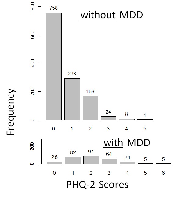
Screening tests include continuous measurements for which there are no “positive” or “negative” results at first (Gordis, 2014), such as the use of the two-item Patient Health Questionnaire (PHQ-2) to screen for major depressive disorder. Thus, we must make decisions on the score above or below which a person would be classified as having a “positive” screening result; otherwise, they will be classified as having a “negative” result. This specific score for categorization is known as the “cut-off level”.
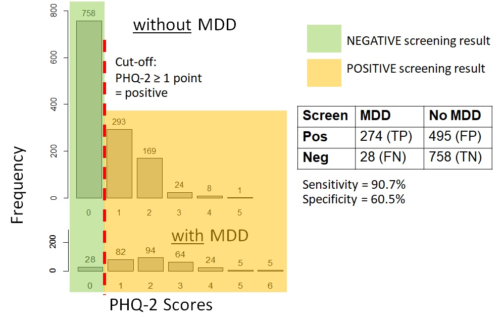
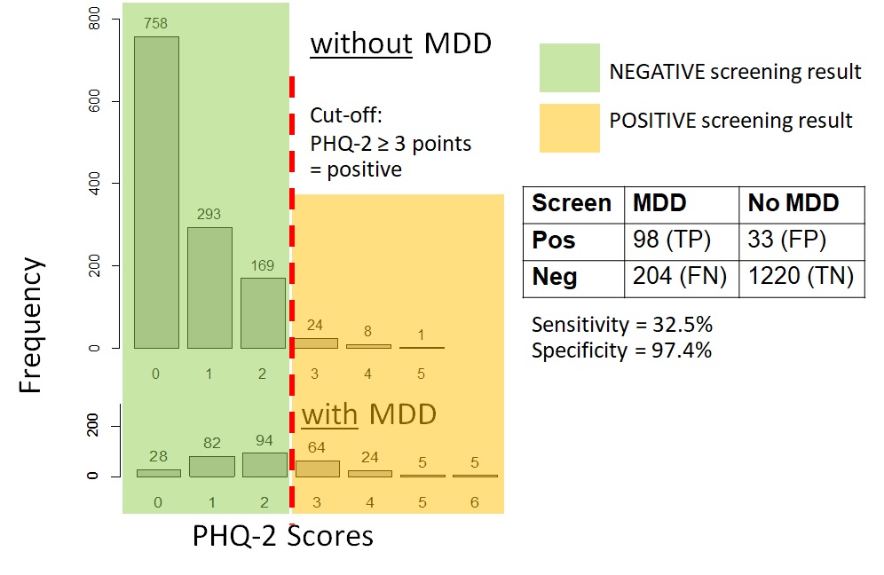
Figure 12.4.1a shows data on the PHQ-2 depression among samples of a community-based population of adults in Thailand with and without clinical depression. For those interested, the hypothetical distributions came from actual screening scores reported by the general population of adults in Thailand in 2021 (Wichaidit et al., 2022) combined with the reported sensitivity and specificity of the PHQ-2 at specific score points (Kroenke et al., 2003). The data set for the analyses can also be found in the Supplementary Section. We can see that there was an overlap in the PHQ-2 scores among those with and without clinical depression. However, those with clinical depression generally had higher PHQ-2 scores than those who did not. Thus, using a relatively low cut-off score on the PHQ-2 would allow us to identify most or all of those with depression (high sensitivity, i.e., few to no false negatives) (Figure 12.4.1b). However, we would have many participants who screened positive but who did not actually have depression (low specificity, i.e., a large number and proportion of false positives). Had we used a relatively high cut-off score, the inverse would have occurred where sensitivity was low (i.e., a large number and proportion of false negatives) but specificity was high (i.e., few to no false positives) (Figure 12.4.1c).
|
a. Distribution of the scores among those without MDD and with MDD |
|
|
|
b. Sensitivity and specificity when screening cut-off was PHQ-2 ≥ 1 point |
|
|
|
c. Sensitivity and specificity when screening cut-off was PHQ-2 ≥ 3 points |
|
|
Remarks: The MDD vs. no MDD categorizations were hypothetical; screening scores are based on data from a previous study (Wichaidit et al., 2022)
As you may notice, the sensitivity and specificity of the screening test vary depending on the cut-off point, and there is a trade-off between sensitivity and specificity (Gordis, 2014). The lower the cut-off point, the higher the sensitivity and the lower the specificity. The higher the cut-off point, the lower the sensitivity and the higher the specificity. Generally, there is no clear-cut answer on the most appropriate cut-off point for a given screening test, and the choice generally depends on the context of the outcome of interest, i.e., the consequence of false positive vs. false negative results, such as the issues pertaining to depression screening mentioned in the previous paragraphs.
12.5 Biases in Screening Tests
Screening programs are meant to detect diseases early and improve the prognosis and quality of life of patients who screened positive and are found to have the disease. However, the evaluation of screening interventions is prone to numerous biases. Most biases make the prognosis among those who were screened appear to be better than those who were unscreened (Szklo & Nieto, 2019). The five main types can be summarized as follows:
* Selection bias. Selection bias in screening evaluations occurs when the screened group significantly differs from the unscreened group (e.g., having a higher socioeconomic status and better disease prognosis). This bias can be overcome by using an experimental study design.
* Incidence-prevalence bias (also known as survival bias). This bias occurs in screening interventions with multiple rounds when the prevalent cases detected in the first round (which generally include those with better than average survival) are compared to incident cases detected in later rounds.
* Length bias. This bias is similar to incidence-prevalence bias and occurs when patients detected by screening seem to have a better prognosis than those detected between screening periods. The term “detectable preclinical phase” (DPCP) refers to the time from the earliest point when the diagnosis of the disease is possible to the point of usual diagnosis due to the appearance of signs and symptoms. Patients detected by screening are more likely to have a disease type with a longer detectable preclinical phase (which generally has a better prognosis) than patients not detected by screening.
* Lead time bias. Lead time is a subset of the detectable preclinical phase and refers to the time from the point when early diagnosis is generally made to the point of usual diagnosis due to the appearance of signs and symptoms. When comparing the prognosis of screened vs. unscreened patients, lead time bias occurs when survival time is measured starting from the point of early diagnosis by screening to the time of the outcome among the screened patients but is measured starting from the usual point of diagnosis among the unscreened patients. A way to minimize this bias is to use the same starting point for the screened patients, i.e., the point of usual diagnosis. However, since the screened patients no longer needed the usual diagnosis and thus the point of usual diagnosis does not occur in this group, an estimate needs to be made according to methods described in a text elsewhere (Szklo & Nieto, 2019).
* Overdiagnosis bias. Overdiagnosis bias refers to bias arising from the diagnosis of patients whose subclinical disease (detected by screening) never becomes clinical, symptomatic, invasive, or lethal. Thus, patients in the screened group who are over-diagnosed contribute to the higher survival time among the screened group yet remain unidentified in the unscreened group.
12.6 Reliability (Repeatability) of Tests
A good screening test is not only one that can clearly distinguish between those who do and do not have the disease but must also be reliable. In epidemiology, reliability refers to the extent to which a test is repeatable, i.e., the extent to which test results obtained can be repeated if the test is repeated (Gordis, 2014). There are many reasons that test results vary, i.e., do not have reliable results, including:
Intrasubject variation (variation within individual subjects): For example, a person’s blood pressure often varies depending on the time of day, physical activity before measurement, and external factors such as medications.
Intra-observer variation (variation in the reading of test results by the same reader): For example, a radiologist reading the same film at two different times may give different results. Generally, the more a test or an examination relies on a human being’s subjective interpretation, the greater the likelihood and extent of intra-observer variation.
Inter-observer variation (variation between those reading the test results): For example, two radiologists reading the same film at the same time may give different answers. Once again, the greater the reliance on human input, the greater the likelihood and extent of variation.
Percentage Agreement
Reliability is an important issue in epidemiological measurement, and epidemiology is a quantitative discipline. Therefore, we need to quantify reliability in the same manner as we measure other things in epidemiology. The simplest measure is percentage agreement: the percentage of identical opinions between two measurements.
Consider, for example, the results of psychosis screening by two psychiatrists in the same group of psychiatric inpatients.
|
|
|
Physician A |
|
|
|
|
|
Psychosis |
No psychosis |
Total |
|
Physician B |
Psychosis |
90 (A) |
40 (B) |
130 (A+B) |
|
|
No psychosis |
10 (C) |
860 (D) |
870 (C+D) |
|
|
Total |
100 (A+C) |
900 (B+D) |
1000 (A+B+C+D) |
Remark: The numbers here are based on an example provided by Columbia University’s Epiville Project (Columbia University, 2012).
Percent agreement can be calculated as follows:
Percent agreement = (A+D) / (A+B+C+D)
= (90 + 860) / (1000)
= 950/1000
= 0.95, or 95%
The two physicians gave the same screening results in 95% of their opinions. This number may appear to be decent at first, but things may look different upon closer scrutiny. If we were to ignore cell D and only focus on the positive screenings, and the agreement thereof, we would obtain the following calculation:
Percent agreement (Modified) = A / (A+B+C)
= 90 / (90 + 40 + 10)
= 90/140
= 0.64, or 64%
In giving a positive screening of psychosis, the two physicians had the same opinion only 64% of the time. So, why was there such a big difference? The answer is in the low prevalence of the disorder. Most of the patients who underwent the screening procedure did not have psychosis. Thus, probabilistically, the two physicians would give negative screening results to most of their clients. These large numbers of negative findings then accounted for the higher percentage agreement in the first calculation (when the number in cell D was included).
Kappa Statistic
An alternative approach to the measurement of agreement (i.e., repeatability or reliability) may be to incorporate chance as part of the measurement. In other words, we can take into consideration the extent to which our observed agreement between the two physicians exceeded that which results just from chance. To do this, we can use the kappa statistic with two questions (Gordis, 2014):
1. How much better is the agreement between the observers’ readings than would be expected by chance alone?
2. What is the most that the two observers could have improved their agreement over the agreement that would be expected by chance alone?
The kappa statistic is expressed as a proportion of maximum improvement that occurred beyond the agreement expected by chance alone (Gordis, 2014). The higher the kappa statistic, the more reliable the measurement. The kappa statistic could be calculated from the following formula:
κ=Pagree_observed-Pexpected_chance100%-(Pexpected_chance)
Generally, a kappa below 0.40 represents poor agreement, a kappa between 0.40 and 0.75 represents fair to good agreement, and a kappa greater than 0.75 represents excellent agreement (Landis & Koch, 1977).
Let us now see how well our two psychiatrists did with their screening work compared to chance alone.
Recall that our observed agreement (Pagree_observed) has already been calculated:
Percent Agreement = (A+D) / (A+B+C+D) = (90 + 860) / (1000) = 0.95, or 95%
The expected agreement (Pagree_expected) can be calculated by multiplying the row and column total of each cell and dividing them by the total population size:
|
|
|
Physician A |
|
|
|
|
|
Psychosis |
No psychosis |
Total |
|
Physician B |
Psychosis |
(130*100)/1000 = 13 |
(130*900)/1000 = 117 |
130 (A+B) |
|
|
No psychosis |
(870*100)/1000 = 13 |
(870*900)/1000 = 783 |
870 (C+D) |
|
|
Total |
100 (A+C) |
900 (B+D) |
1000 (A+B+C+D) |
Expected Agreement = Pagree_expected = (Aexpected + Dexpected) / Total
= (13+783)/1000 = 796/1000 = 0.796 or 79.6%
We then replace the values in the kappa statistic formula:
κ=Pagree_observed-Pexpected_chance100%-(Pexpected_chance)
κ=95.0%-79.6%100%-(79.6%)=15.4%20.4%=0.754
According to the criteria, our kappa statistic of 0.754 indicated a good level of agreement but just barely above the cut-off point (Landis & Koch, 1977).
12.7 Practical Exercises
12.7.1 Practical Exercises Part 1 (coding not required):
Calculate the sensitivity, specificity, positive predictive value, and negative predictive value of the PHQ-2 screening tool for major depressive disorder at the cut-off value where a respondent with a score of 3 points or higher is considered as having a positive screening result based on data in the following table:
|
|
Had major depressive disorder |
Did not have major depressive disorder |
|
Screened Positive |
98 |
33 |
|
Screened Negative |
204 |
1220 |
Show your work.
12.7.2 Practical Exercises Part 2 (coding required):
Note: the data set and supporting file(s) are available at this webpage: https://www.kaggle.com/wichaiditwit/datasets
Using the data set fig_12_4_1.csv, please calculate the sensitivity and specificity of the PHQ-2 at different cut-off points (from 1 point to 6 points).
12.8 Conclusion
Screening is the use of tests on a large scale to identify the presence of disease in apparently healthy people. In this chapter, we have covered the definition and types of screening, the calculation of key measures (sensitivity, specificity, positive predictive value or PPV, and negative predictive value or NPV), potential biases in screening tests, and methods to measure the reliability of screening tests (percentage agreement and kappa statistic). With advancements in artificial intelligence technology and genetic and molecular epidemiology, readers should keep in mind that the issues discussed in this chapter (such as reliability being affected by subjective human input) may eventually become irrelevant; thus, readers should also consult the current literature in epidemiology and diagnostics to stay informed.
References
Bonita, R., Beaglehole, R., & Kjellstrom, T. (2006). Basic Epidemiology (2nd ed.). World Health Organization Press. http://whqlibdoc.who.int/publications/2006/9241547073_eng.pdf
Columbia University. (2012). Epiville: Screening—Data Analysis. Columbia University. https://epiville.ccnmtl.columbia.edu/screening/data_analysis.html
Gordis, L. (2014). Epidemiology (5th edition). Elsevier Saunders.
Kroenke, K., Spitzer, R. L., & Williams, J. B. W. (2003). The Patient Health Questionnaire-2: Validity of a two-item depression screener. Medical Care, 41(11), https://doi.org/10.1097/01.MLR.0000093487.78664.3C
Landis, J. R., & Koch, G. G. (1977). The measurement of observer agreement for categorical data. Biometrics, 33, 159.
Pai, M. (2009). Diagnostic Studies. TeachEpi. https://www.teachepi.org/wp-content/uploads/OldTE/documents/courses/fundamentals/Pai_Lecture13_Diagnostic%20studies.pdf
Szklo, M., & Nieto, F. J. (2019). Epidemiology: Beyond the Basics (4th ed.). Jones & Bartlett Learning.
Taheri Soodejani, M., Tabatabaei, S. M., Dehghani, A., McFarland, W., & Sharifi, H. (2020). Impact of Mass Screening on the Number of Confirmed Cases, Recovered Cases, and Deaths Due to COVID-19 in Iran: An Interrupted Time Series Analysis. Archives of Iranian Medicine, 23(11), 776–781. https://doi.org/10.34172/aim.2020.103
Tulchinsky, T. H., Varavikova, E. A., & Cohen, M. J. (2023). Chapter 3—Measuring, monitoring, and evaluating the health of a population. In T. H. Tulchinsky, E. A. Varavikova, & M. J. Cohen (Eds.), The New Public Health (Fourth Edition) (pp. 125–214). Academic Press. https://doi.org/10.1016/B978-0-12-822957-6.00015-6
Wichaidit, W., Prommanee, C., Choocham, S., Chotipanvithayakul, R., & Assanangkornchai, S. (2022). Modification of the association between experience of economic distress during the COVID-19 pandemic and behavioral health outcomes by availability of emergency cash reserves: Findings from a nationally-representative survey in Thailand. PeerJ, 10, e13307. https://doi.org/10.7717/peerj.13307
Solutions: Practical Exercise, Chapter 12, Part 2
library(epicalc)
setwd(“redacted”)
use(“fig_12_4_1.csv”)
Variable “phq_2_score” is the score we used to screen participants. Variable “depression” is whether the participant actually had depression. We then created the variable “screenpos” to denote participants with positive (1) vs. negative (0) screening results at different cut-off points.
Where the PHQ-2 score of 1 or higher is considered a positive screening result for depression:
screenpos <- ifelse(phq_2_score >= 1, 1, 0)
tabpct(screenpos, depression)
Where the PHQ-2 score of 2 or higher is considered a positive screening result for depression:
screenpos <- ifelse(phq_2_score >= 2, 1, 0)
tabpct(screenpos, depression)
Where the PHQ-2 score of 3 or higher is considered a positive screening result for depression:
screenpos <- ifelse(phq_2_score >= 3, 1, 0)
tabpct(screenpos, depression)
Where the PHQ-2 score of 4 or higher is considered a positive screening result for depression:
screenpos <- ifelse(phq_2_score >= 4, 1, 0)
tabpct(screenpos, depression)
Where the PHQ-2 score of 5 or higher is considered a positive screening result for depression:
screenpos <- ifelse(phq_2_score >= 5, 1, 0)
tabpct(screenpos, depression)
Where the PHQ-2 score of 6 is considered a positive screening result for depression:
screenpos <- ifelse(phq_2_score >= 6, 1, 0)
tabpct(screenpos, depression)
For each cross-tabulation, the calculation of sensitivity and specificity can be made post hoc.
For example, cross-tabulation of depression status with a PHQ-2 score ≥ 3 for a positive screening result yields the following outputs:
Original table
depression
screenpos 0 1 Total
0 1220 204 1424
1 33 98 131
Total 1253 302 1555
In this output, true positives (TP) = 98; false positives (FP) = 33, true negatives (TN) = 1220, false negatives (FN) = 204. Thus:
Sensitivity = TP/(TP+FN) = 98/(98+204) = 32%
Specificity = TN/(TN+FP) = 1220/(1220+33) = 97%
Please repeat the same procedures for all cut-offs, from 1 point to 6 points.
