6 Chapter 6: Case-control Studies

Chapter 6: Case-control Studies

Objectives

After completing this module, you should be able to:

1. Describe the basic principles of case-control studies.

2. Describe common issues encountered in the design and interpretation of findings from case-control studies.

 

6.1 Introduction

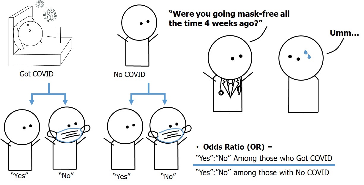
As mentioned in Chapter 3, a case-control study is an observational study that compares the exposure between the cases (members of a population with the outcome of interest) and a comparison group known as the controls (members of a population without the outcome). Case-control studies commonly involve a comparison of the odds of exposure among the cases with the odds of exposure among those of the controls and then a calculation of the ratio between those two odds known as the odds ratio (OR).

Figure 6.1.1 presents an image from Chapter 3 to illustrate the concept of a case-control study on the association between infection with a hypothetical disease called “COVID-26” (as an outcome vs. no infection) and going mask-free four weeks before conducting the study (as an exposure vs. wearing masks). The exposure status was measured by an interview with a healthcare provider. Table 6.1.1 also presents hypothetical data from this study.

Figure 6.1.1 Design of the case-control study on the association between face mask use (or lack thereof) and a hypothetical emerging disease called “COVID-26”

The hypothetical data from the hypothetical case-control study is as follows:

Table 6.1.1 Face mask use among COVID-26 cases and non-cases

	Infected with COVID-26 (Cases, or outcome) (n=200)	Not infected with COVID-26 (Controls, or NO outcome) (n=200)
“Going mask-free” (Exposed)	150 (a)	20 (b)
Used face mask (non-exposed)	50 (c)	180 (d)
Total	200	200

The odds ratio in this study can be calculated as follows:

ODDS of EXPOSURE = (number EXPOSED / number NON-EXPOSED)

Odds ratio (OR) = (Odds of EXPOSURE among CASES) / (ODDS of EXPOSURE among CONTROLS)

OR = (a/c) / (b/d)

=(15050)(20180)=(3)(0.1111)=27.0

In Chapter 3, we mentioned that in case-control studies, we compare the odds of exposure between the cases and the controls, and thus the interpretation needs to follow suit:

“The odds of ‘going mask-free’ among cases of COVID-26 were 27 times higher than among the non-cases (controls) from the same population in Covidia.”

Examples in this chapter (from the chapter as well as other examples) will include exposures that are dichotomous, i.e., participants are classified as being in either the exposed group or the non-exposed group. However, an exposure of interest can be anything, including behaviors (such as not wearing a face mask), dietary intake, contact with a pathogen or a substance, and having certain genes. Thus, the exposure in other case-control studies may be measured from laboratory examination of bodily fluids and tissues in addition to a conventional interview or questionnaire completion. Measurements can also be in nominal scale (e.g., whether someone was going mask-free), ordinal scale (e.g., the number of pregnancies or children), interval scale (e.g., weight, systolic blood pressure), or ratio scale (e.g., waist-to-hip ratio).

 

6.2 Points of Consideration in Designing Case-control Studies

In the author’s own opinion, case-control studies are the most difficult ones to design in epidemiology, as there are multiple aspects to bear in mind with regard to both the design and the interpretation of the study findings, as has been noted elsewhere (Gordis, 2014).

Firstly, unlike cross-sectional studies, case-control studies are not designed to measure the prevalence of the disease of interest. In the example in Figure 6.1.1 and Table 6.1.1, the number of cases and the non-cases (controls) are equal: 200 per group. This occurred because in the study design, for every case of COVID-26, the investigators sampled a comparable individual from the same base population (the population that gave rise to the cases) as the control and conducted interviews regarding their mask-wearing behavior (or lack thereof). In studies of diseases that are very rare, investigators may choose to collect data from more non-cases (controls) to increase the statistical power of the study and rule out chance as the best explanation for the differences in exposure odds between the cases and controls. Thus, some case-control studies may have a case-to-control ratio of 1:2, 1:3, or even 1:4. Cases-to-control ratios beyond 1:4 generally do not convey much additional statistical power relative to the cost incurred to warrant such recruitment.

Secondly, there is an erroneous impression that case-control studies differ from cohort studies in terms of temporal direction: cohort studies go forward in time, whereas case-control studies go backward in time and may be incorrectly referred to as “retrospective studies“ (Gordis, 2014). This distinction is incorrect, as the main difference is in the comparisons. Case-control studies compare the odds of exposure between the cases (those with the outcome) and the controls (those from the same base population as the cases who do not have the outcome). Cohort studies compare the risk of the outcome between individuals in the same source population who have the exposure vs. those who did not have the exposure. More details regarding cohort studies can be found in Chapter 7.

Thirdly, the source of the cases may affect the generalizability of the study findings (Gordis, 2014). Case-control studies can recruit the cases from several sources, including community hospitals, general hospitals, and tertiary hospitals. However, as modern healthcare systems refer more severely ill patients to tertiary facilities, the findings from case-control studies at tertiary hospitals may not be readily generalizable to patients at primary healthcare facilities.

6.2.1 Potential Sources of Selection Bias in Case-Control Studies

Selection bias occurs when the selection and enrollment processes of the study participants contain systematic errors that mean their findings deviate from the truth. Case-control studies involve the selection of the cases and the controls; thus, selection bias can occur when the selection process results in the comparison groups no longer being from the same source population (Gordis, 2014):

Bias potentially introduced by the selection of cases. When designing case-control studies, investigators can generally use either newly diagnosed cases (known as incident cases) or previously diagnosed cases receiving longer-term treatment and disease management (known as prevalent cases). The use of incident cases is preferable because when the exposure of interest is associated with survival, the prevalent cases may be survivors who have the exposure of interest as the other cases without the exposure will have died. The exposure odds among the prevalent cases could be overestimated when compared to incident cases. Thus, the use of incident cases may be preferable to the use of prevalent cases (Gordis, 2014). In that regard, in hospital-based case-control studies, investigators only recruit patients who present themselves at the hospital as cases. Therefore, the exposure measured may not reflect the exposure among patients who had not come to the study hospitals and thus may present an additional source of selection bias.

Bias potentially introduced by the selection of controls. If the author were to identify one area where one needs to exercise the utmost care in study design to reduce the possibility of selection bias, it would be the selection of control group participants for case-control studies. Control participant selection requires thinking with a counterfactual model: the control group participants must reflect the exposure among those who are from the same population as the cases and could have become the cases but did not. This concept is easy to state but very difficult to implement.

The use of hospitalized controls (i.e., patients at the study hospital who do not have the disease of interest) can introduce bias if the disease or condition of the potential control group patients affects the exposure (Gordis, 2014). For example, in a study on pancreatic cancer (as the outcome) and coffee consumption (as the exposure), the investigators found a statistically significant positive association between pancreatic cancer and coffee consumption. The control group participants in the study were selected from the patients of the physicians who treated the cases but had diagnoses other than pancreatic cancer. As the physicians who treated pancreatic cancer patients worked in the gastroenterology clinic, the non-cancer patients in the clinic who became the controls tended to have digestive issues and were either advised by their physicians to reduce coffee consumption or voluntarily reduced coffee consumption in the hope of alleviating the symptoms. Coffee consumption in such control patients was likely lower than coffee consumption in the base population, and the association between pancreatic cancer and coffee consumption could thus have been biased and overestimated (Pai & Kaufman, 2019).

Investigators can also choose to use non-hospitalized controls, such as patients receiving preventive services, friends and families of the cases, or even randomly selected members of the same community as the cases without the disease of interest. However, there are several issues with regard to feasibility (Gordis, 2014). Patients receiving preventive services may have gone through different referral systems compared to the cases, and thus their exposure might not reflect that in the base population which gave rise to the cases. Friends and family members are easy to recruit but may have a similar level of risk behaviors (such as smoking, drinking, and drug use) as the cases, which reduces the researchers’ ability to assess the extent to which an outcome is associated with such risk behaviors (Setia, 2016). Randomly selected community members generally have a low level of willingness to talk to strangers and participate in an epidemiological study with long interviews (Gordis, 2014), particularly when there are simultaneous work and family concerns. Community members who agreed to participate may have a distribution of exposure that does not reflect the exposure distribution in the base population that gave rise to the cases.

6.2.2 Potential Sources of Information Bias in Case-Control Studies

In addition to the way in which participants are selected for the comparison groups (particularly the controls), the collection of information in case-control studies can also introduce information bias into the study findings. Such bias is common when data regarding past exposure are obtained by interviewing study participants, and it will be the focus of this sub-section. The form of information bias that is particularly common in case-control studies is recall bias: systematic errors arising from differences between the cases and the controls in the accuracy or completeness of recalled past experiences (Porta, 2008). The cases tend to have suspicions about the potential causes of the outcome disease (Gordis, 2014). If the exposure of interest is aligned with the cases’ pre-existing suspicions regarding the potential causes of the outcome disease, the cases would be more likely to recall past exposures than the control, thus biasing the association.

A related source of information bias, which is commonly mistaken for recall bias, is imperfect recall (Luby & Southern, 2017). Epidemiologists who conduct case-control studies of diseases with a long manifestation period (such as pancreatic cancer) may ask participants to describe their coffee consumption habits two decades prior to the study interview, as this period could be the relevant window of exposure in which coffee’s potential biological effect on pancreatic tissue first took place. However, humans tend to forget or incorrectly recall past behaviors; thus, some participants might have over-reported their coffee consumption two decades prior, whereas others might have under-reported it. If there is a systematic tendency to over-report or under-report past exposure due to imperfect recall, then imperfect recall could have introduced information bias into the study findings. Yet, imperfect recall does not necessarily lead to bias (Luby & Southern, 2017), particularly when misclassifications from imperfect recall occur at random and do not lead the observed findings to deviate from the truth.

Case-control studies can also be affected by social desirability bias, particularly when the exposure of interest is not socially desirable, illegal, or a source of embarrassment. Study participants may also answer questions in a way that addresses the need to maintain or enhance their self-esteem and introduces self-serving bias into the study findings. Lastly, participants may give affirmative answers or agree with given statements in a way that does not align with their actual feelings, influenced by the human tendency to be agreeable, known as acquiescence bias. Lastly, in addition to the participants, the investigators can also become a source of bias, most commonly through the introduction of observer bias. The details of this are available in Chapter 9: Bias.

6.2.3 Comparison between Cross-sectional and Case-control Studies

Cross-sectional and case-control studies differ in purpose, study design, advantages, and disadvantages. However, they also share similarities regarding measurement and certain potential sources of information bias. A summary of the comparison can be found in Table 6.2.3.1 below.

Table 6.2.3.1 Comparison of cross-sectional and case-control studies

Component	Cross-sectional studies	Case-control studies
Purpose	* Estimate prevalence of exposures and outcomes of interest	* To assess the extent to which an outcome is associated with an exposure
Design	* Sample participants from members of the population of interest and measure their exposure and outcome status	* Select participants with the outcome of interest (preferably those who just developed the outcome, also known as “incident cases”) * Then, select members of the base population that gave rise to the cases who have not become the cases as the “controls”
Measuring the exposure prevalence	* Can measure the prevalence of multiple exposures simultaneously	* Generally, not appropriate for measuring the prevalence of exposures of interest in the general population
Measuring outcome prevalence	* Can measure the prevalence of multiple outcomes simultaneously	* Cannot measure the prevalence of the outcome
Use in the study of rare exposures	* Not appropriate if conducted in the general population	* Not appropriate
Use in the study of rare outcomes	* Not appropriate	* Appropriate
Common measure(s) of association	* Odds ratio (the ratio of the odds of the outcome among the exposed vs. non-exposed, or vice versa)	* Odds ratio (the ratio of the odds of the exposure among the cases vs. the controls)
Common source(s) of selection bias	* Non-response (refusal to participate)	* Control selection, resulting in the exposure odds among the control not reflecting that of the base population that gave rise to the cases * Non-response
Common source(s) of information bias	* Social desirability bias * Self-serving bias * Response acquiescence bias * Observer bias	* Recall bias * Social desirability bias * Self-serving bias * Response acquiescence bias * Observer bias
Use of the study findings	* Monitoring of trends in a population * Generate hypotheses for further studies	* Identify potential determinants of a rare disease * Generate hypotheses for further studies

6.2.4 Nested Case-Control Study

When there is a new laboratory technique that can be used to gain insights from stored biospecimen, but the technique is too expensive to be used on all of these biospecimens, investigators can opt to conduct a nested case-control study, defined as “…an important type of case-control study in which cases and controls are drawn from the population in a fully enumerated cohort” (Porta, 2008). In nested case-control studies, the outcome vs. no outcome status is ascertained in the follow-up period (i.e., at the time of study). Since data on the exposure and other characteristics of the participants are recorded at baseline, the nested design can help reduce potential exposure misclassification and recall bias. Furthermore, as members of a cohort come from the same base population, the cases in nested case-control studies can be cohort members with the outcome at follow-up, whereas the controls can simply be members of the cohort without the outcome at follow-up. In that regard, nested case-control studies are vulnerable to selection bias if there is a differential loss to follow-up between cohort members who became the cases and those who became the controls.

6.3 Example of Case-Control Studies

Investigators (del Mar Fernández et al., 2019) conducted a case-control study to identify potential determinants of premenstrual syndrome (PMS) and premenstrual dysphoric syndrome (PMDD) with incident cases of PMS and PMDD recruited from health facilities in Spain and controls recruited from women who consulted the same health facilities for other motives (e.g., screening for uterine cancer, contraception counseling, or fertility).

Gynecologists and midwives helped the investigators to recruit the patients, who then completed anonymous, voluntary, self-administered questionnaires including the presence or absence of PMS and PMDD, perceived psychological stress during the three months before the study, neuroticism, and other demographic and clinical-psychological characteristics (coping style, sleep hours, sleep satisfaction, age at menarche, etc.). Investigators divided participants into quartiles according to their perceived stress scores and neuroticism scores. Investigators then assessed the extent to which PMS and PMDD case status were associated with various characteristics using conditional logistic regression. For the purpose of this sub-section, only the association of PMDD case status vs. stress and neuroticism will be displayed and described (Table 6.3.1).

Table 6.3.1 Associations between premenstrual dysphoric syndrome (PMDD) and perceived stress (in quartiles) and neuroticism (in quartiles)

Characteristic	Cases (Participants with PMDD) (n = …)	Controls (Participants without PMDD) (n = …)	Unadjusted OR (95% CI)	Adjusted OR* (95% CI)
Perceived stress level
1st quartile (Lowest)	16 (18.8%)	65 (38.2%)	Reference	Reference
2nd quartile (Lower)	8 (9.4%)	40 (23.5%)	0.78 (0.29, 2.12)	0.83 (0.29, 2.32)
3rd quartile (Higher)	23 (27.1%)	42 (24.7%)	2.59 (1.12, 6.00)	2.53 (1.06, 6.06)
4th quartile (Highest)	38 (44.7%)	23 (13.5%)	8.93 (6.63, 21.98)	8.05 (3.07, 21.12)
Neuroticism level
1st quartile (Lowest)	10 (12.7%)	42 (27.6%)	Reference	Reference
2nd quartile (Lower)	18 (22.8%)	56 (36.8%)	1.46 (0.54, 3.97)	1.80 (0.64, 5.06)
3rd quartile (Higher)	21 (26.6%)	24 (15.8%)	3.58 (1.29, 9.98)	3.70 (1.27, 10.77)
4th quartile (Highest)	30 (38.0%)	30 (19.7%)	5.75 (2.08, 15.84)	5.73 (1.96, 16.77)

Bold numbers denote statistical significance at a 95% level of confidence.

* Adjusted for sleep hours, sleep satisfaction, and age at menarche.

Adapted from del Mar Fernández et al., 2019

Both perceived stress and neuroticism were associated with PMDD, particularly at higher and highest levels. The cases had an 8 times higher odds of having perceived stress at the 4th quartile (highest) than the controls, and the association remained statistically significant after adjusting for potential confounders (45% vs. 14%, Adjusted OR = 8.05; 95% CI = 3.07, 21.12). The cases also had over 4 times higher odds of having neuroticism at the 4th quartile (highest) than the controls, and the association remained statistically significant after adjusting for potential confounders (38% vs. 20%, Adjusted OR = 5.73; 95% CI = 1.96, 16.77).

In the Discussion section, the investigators made the following remarks regarding potential reverse causation. It is possible that although the PMDD was incident and measured at recruitment, participants could have developed a less intense form of PMDD before the onset of stress and neuroticism. Investigators noted the potential for recall bias, i.e., the cases being more likely to report high levels of stress and neuroticism than the controls, albeit at a low likelihood.

“Our study was a case-control study in which cases of PMS/PMDD were incident. Theoretically, the levels of perceived stress, neuroticism and coping refer to a time window that precedes the onset of the syndrome. However, it is not unlikely that the premenstrual symptoms, albeit in a less intense form, were concomitant to the assessment of psychological factors. A reverse causation process, in which the presence of premenstrual symptoms produces stress and inadequate coping strategies, cannot be ruled out. This could explain the fact that high levels of certain adaptive coping strategies, expected to reduce the odds of PMS/PMDD, were eventually associated with a large increase in the odds risk.

“Furthermore, as in any case-control study, our study may be subject to recall bias. PMS/PMDD cases may better assess their psychological factors than controls. However, this is unlikely to occur as the participants were not aware of the hypothesis of the study. Indeed, the hypothesis of a relation between psychological factors and premenstrual syndrome was not disclosed to the participants, as these factors were only part of a long list of exposure factors that have been assessed in the questionnaire.”

(del Mar Fernández et al., 2019, p. 10).

 

6.4 Practical Exercise

Note: the data set and supporting file(s) are available at this webpage: https://www.kaggle.com/wichaiditwit/datasets

Please note that this exercise is recommended but optional. I wish to invite the reader to read this section carefully, as it contains instructions on how to analyze the exercise data set. The solution to the exercise is available at the very end of this chapter after the references.

Assignment: Read the following analysis plan, adapted from a published case-control study (Bhatt et al., 2018), and complete the table at the end of this section.

Source: Bhatt, M., Perera, S., Zielinski, L., Eisen, R. B., Yeung, S., El-Sheikh, W., DeJesus, J., Rangarajan, S., Sholer, H., Iordan, E., Mackie, P., Islam, S., Dehghan, M., Thabane, L., & Samaan, Z. (2018). Profile of suicide attempts and risk factors among psychiatric patients: A case-control study. PLOS ONE, 13(2), e0192998. https://doi.org/10.1371/journal.pone.0192998

 

Title: Association between attempted suicide and borderline personality disorder among psychiatric patients in Canada

Objective: To assess the extent to which attempted suicide is associated with borderline personality disorder among psychiatric patients in Canada

Methods

The complete methodology of this study (Bhatt et al., 2018) and the data file can be found at this link: https://journals.plos.org/plosone/article?id=10.1371/journal.pone.0192998

Abridged details are provided below.

Study design and setting

The investigators conducted a case-control study titled the Study of Determinants of Suicide Conventional and Emergent Risk (DISCOVER) in Hamilton, Ontario, Canada. The study data were collected at St. Joseph’s Healthcare and Hamilton Health Sciences Hospital.

Study population and participants

Case group participants included adult psychiatric inpatients (aged 18 years or older) who made a suicide attempt (self-directed injury with the specific intent to die) that necessitated admission to a medical or psychiatric ward. The cases included those who made a suicide attempt within three months of recruitment (case-recent group) and those who had a lifetime history of attempted suicide (case-past group). For this analysis, the case-recent and case-part groups are combined into one “case” group. The control group participants included patients admitted to the same psychiatric hospital within the same time frame as the cases but who had never attempted suicide. The investigators did not match the cases and the controls with regard to age and sex (although this was initially planned).

Participant recruitment and data collection:

Clinical staff identified eligible hospitalized patients and informed trained research assistants, who approached the patients and inquired whether they would be interested in participating in the study. All participants provided written informed consent before data collection. The research assistants then collected data via face-to-face interviews with structured questionnaires.

Study Variables

Variable	Definition	Coding
Exposure: Borderline personality disorder	Use the variable bsl_total (the total score for the 23-item Borderline Symptoms List Score), divide the number by 23, and use 1.50 or higher as the cut-off point for borderline personality disorder (BPD). Having an average score of 1.5 or higher in the BSL-23 is deemed to be an appropriate cut-off point for borderline personality disorder (BSD) (NovoPsych, 2022). As such, we will use the same cut-off point to categorize the participants as either exposed (BPD) or non-exposed (no BPD).	bsl_average <- bsl_total/23 bpd <- ifelse(bsl_average>=1.50, 1, 0)
Outcome: Suicide attempt	Variable “allcasepsych” with values 1 (cases) vs. 0 (controls) History of making a suicide attempt that necessitated admission to a medical or psychiatric ward. For this analysis, the case-recent and case-part groups are combined into one “case” group.	case <- allcasepsych
Confounders
Age of the patient	The variable “age” seems to contain the age of the participants. This variable will be used in the analysis as it appears.	Variable “age”
Sex of the patient	The variable “sex” seems to contain dichotomous discrete values and will be used in the analysis as it appears.	Variable “sex”
High impulsiveness (vs. moderate to low impulsiveness)	The investigators used the 30-item Barratt Impulsiveness Scale (BIS-11) to measure impulsiveness. The scale yielded impulsiveness values that could range from 30 points to 120 points. The BIS-11 actually has no defined cut-off point but perhaps a score of 72 or higher would be an appropriate cut-off point as has been used in a recent study (Palmu et al., 2019) and aligns with the findings from a review of the use of the tool during the past 50 years (Stanford et al., 2009).	#Create a variable ‘impulsiveness_high’ from the BIS score at the cut-off of 72 points or higher #The variable ‘bis_total’ contains what seems to be the BIS-11 score and thus is used for the analyses impulsiveness_high <- ifelse(bis_total>=72, 1, 0)

Study Instruments

The study instrument is a structured interview questionnaire, the content of which included sociodemographic characteristics, intention to die as a result of the suicide attempt, the Barratt Impulsiveness Scale (BIS), the Borderline Symptom List (BSL), and the Mini International Neuropsychiatric Interview (M.I.N.I.).

Data Analysis

We will use bivariate analysis with cross-tabulation (column percentage) to present descriptive analyses. We will then use univariable and multivariable logistic regression to measure the association between the exposure and the outcome. Previous studies have found that factors associated with suicide include age (Wu et al., 2021), sex (Wu et al., 2021), and impulsivity (Bruno et al., 2023; Gvion et al., 2015). Thus, we decided to include these variables as the confounders in the multivariable logistic regression analyses.

Ethical Considerations

The investigators stated in the article: “The study procedures were approved by the Hamilton Integrated Research Ethics Boards (HIREB) (REB number 10–661 for St. Joseph’s Healthcare Hamilton and 11–3479 for Hamilton Health Sciences Hospitals).”

Table 6.4.1 Prevalence of borderline personality disorder (exposure) among the cases and the controls

Borderline Personality Disorder	Cases (Suicidal attempt) (n = …)	Controls (No suicidal attempt) (n = …)	Unadjusted OR (95% CI)	Adjusted OR (95% CI)
No borderline personality disorder (BSL < 1.50 points)			1 (Reference)	1 (Reference)
Borderline personality disorder (BSL ≥ 1.50 points)

*Adjusted for age, sex, and high impulsiveness.

6.5 Conclusion

A case-control study is an observational study that compares the exposure between the cases (members of a population with the outcome of interest) and a comparison group known as the controls (members of a population without the outcome). The most common measure of association in case-control studies is the odds ratio (OR), calculated by dividing the odds of exposure among the cases by the odds of exposure among the controls.

The most common source of selection bias in case-control studies is the selection of controls that do not come from the base population that gave rise to the cases, resulting in ORs that systematically deviate from the truth. One source of potential information bias that is very particular to case-control studies is recall bias, in which the cases are more likely to recall past exposure to the controls and do so more accurately due to their existing hypotheses of the etiology of their illness. Other sources of information bias include social desirability bias, self-serving bias, and response acquiescence bias. Despite the limitations, the case-control study design is useful in the investigation of rare diseases, and the findings can be used to generate hypotheses for further investigations.

References

Bhatt, M., Perera, S., Zielinski, L., Eisen, R. B., Yeung, S., El-Sheikh, W., DeJesus, J., Rangarajan, S., Sholer, H., Iordan, E., Mackie, P., Islam, S., Dehghan, M., Thabane, L., & Samaan, Z. (2018). Profile of suicide attempts and risk factors among psychiatric patients: A case-control study. PLOS ONE, 13(2), e0192998. https://doi.org/10.1371/journal.pone.0192998

Bruno, S., Anconetani, G., Rogier, G., Del Casale, A., Pompili, M., & Velotti, P. (2023). Impulsivity traits and suicide related outcomes: A systematic review and meta-analysis using the UPPS model. Journal of Affective Disorders, 339, 571–583. https://doi.org/10.1016/j.jad.2023.07.086

del Mar Fernández, M., Regueira-Méndez, C., & Takkouche, B. (2019). Psychological factors and premenstrual syndrome: A Spanish case-control study. PLOS ONE, 14(3), e0212557. https://doi.org/10.1371/journal.pone.0212557

Gordis, L. (2014). Epidemiology (5th Edition). Elsevier Saunders.

Gvion, Y., Levi-Belz, Y., Hadlaczky, G., & Apter, A. (2015). On the role of impulsivity and decision-making in suicidal behavior. World Journal of Psychiatry, 5(3), 255–259. https://doi.org/10.5498/wjp.v5.i3.255

Luby, S., & Southern, D. (2017, August). The Pathway to Publishing: A Guide to Quantitative Writing in the Health Sciences. https://globalhealth.stanford.edu/wp-content/uploads/2019/07/A-Guide-to-Quantitative-Scientific-Writing-V-23.pdf

NovoPsych. (2022, June 24). Borderline Symptom List (BSL-23). https://novopsych.com.au/wp-content/uploads/2022/06/bsl-23-borderline-symptoms-assessment-report-3.pdf

Pai, M., & Kaufman, J. S. (2019). Bias File 2. Should we stop drinking coffee? The story of coffee and pancreatic cancer. TeachEpi. https://www.teachepi.org/wp-content/uploads/OldTE/documents/courses/bfiles/The%20B%20Files_File2_Coffee_Final_Complete.pdf

Palmu, R., Partonen, T., Suominen, K., & Vuola, J. (2019). Impulsiveness and burn patients. Burns, 45(1), 63–68. https://doi.org/10.1016/j.burns.2018.08.017

Porta, M. (Ed.). (2008). A Dictionary of Epidemiology (5th ed.). Oxford University Press.

Setia, M. S. (2016). Methodology Series Module 2: Case-control Studies. Indian Journal of Dermatology, 61(2), 146–151. https://doi.org/10.4103/0019-5154.177773

Stanford, M. S., Mathias, C. W., Dougherty, D. M., Lake, S. L., Anderson, N. E., & Patton, J. H. (2009). Fifty years of the Barratt Impulsiveness Scale: An update and review. Personality and Individual Differences, 47(5), 385–395. https://doi.org/10.1016/j.paid.2009.04.008

Wu, Y., Schwebel, D. C., Huang, Y., Ning, P., Cheng, P., & Hu, G. (2021). Sex-specific and age-specific suicide mortality by method in 58 countries between 2000 and 2015. Injury Prevention : Journal of the International Society for Child and Adolescent Injury Prevention, 27(1), 61–70. https://doi.org/10.1136/injuryprev-2019-043601

 

Solutions: Practical Exercise for Chapter 6 (Case-Control Studies)

Open the epicalc package and the data file.

library(epicalc)

setwd(“[redacted]”)

use(“Ch6_exercise.csv”)

Exposure: Borderline personality disorder

Use the variable bsl_total (the total score for the 23-item Borderline Symptoms List Score), divide the number by 23, and use 1.50 or higher as the cut-off point for borderline personality disorder (BPD).

Having an average score of 1.5 or higher in the BSL-23 is deemed an appropriate cut-off point for borderline personality disorder (BSD) (NovoPsych, 2022). As such, we will use the same cut-off point to categorize the participants as either exposed (BPD) or non-exposed (no BPD).

bsl_average <- bsl_total/23

bpd <- ifelse(bsl_average>=1.50, 1, 0)

Outcome: Suicide attempt

Variable “allcasepsych” with values 1 (cases) vs. 0 (controls)

The history of making a suicide attempt that necessitated admission to a medical or psychiatric ward. For this analysis, the case-recent and case-part groups are combined into one “case” group.

case <- allcasepsych

Confounders

Using variables “age” and “sex” as they appear.

High impulsiveness (vs. moderate to low impulsiveness)

Create a variable “impulsiveness_high” from the BIS score at the cut-off of 72 points or higher.

The variable “bis_total” contains what seems to be the BIS-11 score and thus is used for the analyses.

impulsiveness_high <- ifelse(bis_total>=72, 1, 0)

Filling in Table 6.3.1

For prevalence of borderline personality disorder (exposure) among the cases and the controls, we use bivariate analysis with cross-tabulation (column percentage) to present descriptive analyses.

Make sure to use column percentage, and be mindful that in our table, the cases are to the left and the non-cases are to the right.

tabpct(bpd, case)

We then use univariable and multivariable logistic regression to measure the association between the exposure and the outcome.

Previous studies have found that factors associated with suicide include age (Wu et al., 2021), sex (Wu et al., 2021), and impulsivity (Bruno et al., 2023; Gvion et al., 2015). Thus, we decided to include these variables as the confounders in the multivariable logistic regression analyses.

Univariable logistic regression:

model1 <- glm(case ~ bpd, family=binomial)

logistic.display(model1)

Multivariable logistic regression with adjustments for age, sex, and having high impulsiveness:

model2 <- glm(case ~ bpd + age + sex + impulsiveness_high, family=binomial)

logistic.display(model2)