8 Chapter 8 – Risk and Return

8.1 Introduction to Risk and Return

8.1.1 Concept Overview:

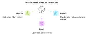
In finance, the concept of risk and return lies at the heart of investment decision-making. Every investment carries some degree of risk, and understanding this risk is essential to assess whether the potential return justifies it. Broadly speaking, higher risk is associated with the potential for higher returns, and lower risk tends to lead to lower expected returns. This relationship forms the foundation for managing investments, evaluating financial opportunities, and ultimately maximizing shareholder value.

8.1.2 Key Points to Address in This Section:

1. 1. Definition of Risk: Explain risk as the chance of earning less than the expected return.
   2. Expected Return: Introduce the notion of expected return as an average or anticipated return based on probability.
   3. Types of Risk: Highlight the major categories of risk, such as general economic factors (like inflation or interest rate changes) and firm-specific factors (like product success or management decisions).

8.2 Defining and Measuring Risk

8.2.1 Concept Overview:

Risk is a central concept in finance, describing the likelihood that an investment’s actual return will differ from its expected return. Evaluating risk involves analyzing two critical dimensions: the probability of different outcomes and the magnitude of potential unfavorable results. These factors help investors assess whether a particular investment aligns with their financial goals and risk tolerance.

The financial interpretation of risk extends beyond simply losing money. Any deviation from the expected return—whether above or below—contributes to risk. For example, an investment failing to meet expected returns, even if it generates a small positive return, still carries a degree of risk. Therefore, comprehensive risk evaluation includes the potential for lower-than-anticipated returns, significant losses, or unfulfilled financial objectives.

8.2.2 Key Topics:

1. Probability and Magnitude of Outcomes

Both the probability and magnitude of potential results are integral to understanding risk. An event with a high probability but low impact might be considered less risky than one with a lower probability but a significant potential loss.

• • Probability quantifies the likelihood of an outcome. For example, a 90% probability of success indicates more certainty than a 10% probability.
  • Magnitude measures the size of the outcome. An event with a small potential loss is less risky than one with a high potential loss, even if their probabilities are the same.

2. Types of Risk Factors

To effectively manage risk, understanding its sources is essential. Risks in finance can be broadly categorized into two types: economic (market) risks and firm-specific risks.

Economic or Market Risk Factors: These risks stem from overall economic conditions and typically affect all securities to some extent.

• • Examples include inflation, interest rate fluctuations, currency exchange volatility, and political instability.
  • Market risks are considered systematic risks, meaning they cannot be mitigated through diversification.

Firm-Specific or Idiosyncratic Risks: These risks are unique to a particular company or industry and can often be reduced through diversification.

• • Examples include product recalls, leadership changes, and lawsuits.
  • Since these risks impact only specific firms, they are referred to as diversifiable risks.

3. Quantifying Risk with Expected Return

In finance, risk is often quantified in terms of potential returns, specifically by calculating the expected return, which averages all possible outcomes weighted by their probabilities.

Formula for Expected Return:

[latex]E(R) = \sum (P_i \times R_i)[/latex]

Where:

• • [latex]P_i[/latex] = Probability of outcome i
  • [latex]R_i[/latex] = Return of outcome i

8.3 Probability Distributions, Expected Return, and Standard Deviation for a Single Security

When evaluating an investment, it’s crucial to understand the range of possible outcomes and the likelihood of each. This is where probability distributions, expected return, and standard deviation come into play, helping investors gauge both the potential return and risk of a security.

8.3.1 Probability Distributions

A probability distribution is a statistical function that describes all possible outcomes of an investment and the likelihood of each. In finance, these distributions help model the range of returns for a security.

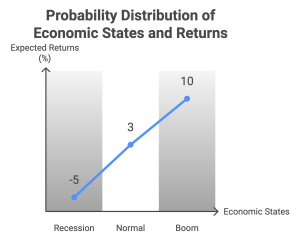
For example, imagine a stock whose returns depend heavily on market conditions. A simple probability distribution might look like this:

State of Economy Probability Return (%)

• • • Recession has a 20% probability with a -10% return.
    • Stable Growth has a 50% probability with a 5% return.
    • Boom has a 30% probability with a 15% return.

Each state is assigned a probability that represents the likelihood of that state occurring, and the returns are the outcomes associated with each state.

8.3.2 Expected Return

The expected return is a weighted average of all possible returns, where weights correspond to each outcome’s probability. It represents the average return expected over an infinite number of similar investments under the same conditions.

The formula for expected return ( E(R) ) is:

[latex]E(R) = \sum (P_i \times R_i)[/latex]

where:

• • • [latex]P_i[/latex] = Probability of outcome i
    • [latex]R_i[/latex] = Return of outcome i

Using the above example:

[latex]E(R) = (0.20 \times -10\%) + (0.50 \times 5\%) + (0.30 \times 15\%) = -2\% + 2.5\% + 4.5\% = 5\%[/latex]

This 5% expected return represents the average return you might expect from this investment over time.

8.3.3 Standard Deviation

The Standard Deviation measures the variability or volatility of returns from the expected return, quantifying the investment’s risk. A higher standard deviation means the returns are more spread out, indicating greater risk.

To calculate the standard deviation of returns ([latex]\sigma[/latex] ):

1. 1. 1. Subtract the expected return from each possible return to find the deviation for each outcome.
      2. Square each deviation.
      3. Multiply each squared deviation by the probability of its corresponding outcome.
      4. Sum all the weighted squared deviations.
      5. Take the square root of the result.

The formula for standard deviation ( \sigma ) is:

[latex]\sigma = \sqrt{\sum P_i (R_i - E(R))^2}[/latex]

Using our example:

1. Deviation from Expected Return:

• • • Recession: -10% – 5% = -15%
    • Stable Growth: 5% – 5% = 0%
    • Boom: 15% – 5% = 10%

2. Square each deviation:

• • • Recession: (-15%)^2 = 225%
    • Stable Growth: 0^2 = 0
    • Boom: (10%)^2 = 100%

3. Multiply each by its probability:

• • • Recession: 0.20 x 225 = 45%
    • Stable Growth: 0.50 x 0 = 0
    • Boom: 0.30 x 100 = 30%

4. Sum the results: 45% + 0 + 30% = 75%

5. Square root of the sum: sqrt(75%) = 8.66%

This 8.66% standard deviation means that the investment’s return typically deviates by about 8.66% from the expected return of 5%, indicating the level of risk.

8.3.4 Interpretation of Expected Return and Standard Deviation

• • The Expected Return is a valuable indicator of potential profitability. A higher expected return suggests the investment may be more lucrative, though it’s not a guaranteed outcome.
  • The Standard Deviation reflects the risk or volatility of the investment. An investment with a high standard deviation is riskier but might also offer higher returns.

For instance:

• • A low-risk bond might have an expected return of 3% and a standard deviation of 2%.
  • A growth stock might have an expected return of 12% with a standard deviation of 25%, indicating a wider range of potential outcomes.

By analyzing both expected return and standard deviation, investors can make more informed decisions based on their risk tolerance and investment goals.

8.4 Correlation and Portfolio Risk

Correlation is a critical concept when examining multiple investments in a portfolio, as it measures the degree to which two securities move in relation to each other. Understanding correlation can help investors reduce overall risk through diversification.

8.4.1 What is Correlation?

Correlation quantifies how two investments are related in terms of their returns. It can range from -1 to +1, where:

• • +1 (Perfect Positive Correlation): Both securities move in the same direction with equal proportion. If one stock increases by 10%, the other will also increase by 10%.
  • -1 (Perfect Negative Correlation): The securities move in opposite directions. If one stock rises by 10%, the other falls by 10%.
  • 0 (No Correlation): No predictable relationship exists between the movements of the two securities.

Most real-world securities are not perfectly correlated. Their correlation typically lies somewhere between 0 and +1 due to common influences like the economy, though they are also impacted by individual factors that create differences in their returns.

8.4.2 Examples of Correlated Securities

To illustrate correlation, consider these examples:

• • • High Positive Correlation: Shares of two companies in the same industry, like Coca-Cola and Pepsi, often show a positive correlation. Because they’re in the same sector, factors that affect one—like changes in consumer preferences for soft drinks—are likely to impact the other similarly.
    • Low Positive Correlation: Consider a tech company like Apple and a consumer goods company like Procter & Gamble. These firms operate in different sectors with distinct customer bases and market drivers. Therefore, their correlation is likely positive but low.
    • Negative Correlation: A bond and a stock may exhibit negative or low correlation because bonds are generally safer, fixed-income assets that often rise in value when stocks decline due to their lower risk appeal during economic downturns.

8.4,3 Why Correlation Matters in a Portfolio

The goal of a well-diversified portfolio is to balance risk and return by holding securities that do not all move together. Here’s why correlation is important:

1. 1. 1. Reduces Overall Risk: By combining assets with low or negative correlations, an investor can achieve more consistent returns. When one asset’s return is down, another might be up, smoothing out the portfolio’s performance.
      2. Improves Return Potential Without Adding Excessive Risk: Investors can include higher-risk assets with potential for high returns while balancing them with assets that tend to be more stable, improving the chance for gains without taking on disproportionate risk.

8.4.4 Practical Application of Correlation: Building a Diversified Portfolio

For example, consider an investor constructing a portfolio with 60% stocks and 40% bonds. Stocks and bonds are generally low to negatively correlated, meaning that if the stock market falls, bonds may hold steady or increase in value. This mix could provide a smoother return over time compared to an all-stock portfolio.

Example of Portfolio Construction Using Correlation:

Imagine two stocks, A and B, with an expected return of 8% each.

• • Stock A has a standard deviation of 15% and Stock B a standard deviation of 20%.
  • The correlation between their returns is 0.2 (low positive).

When calculating the expected return and standard deviation of a portfolio comprising both stocks, the positive but low correlation would result in a lower overall portfolio risk compared to holding either stock individually.

Interpreting Correlation in Investment Decisions

• • High Correlation: If two assets are highly correlated, they are likely to experience similar performance, both up and down. This does not reduce portfolio risk and may lead to higher volatility.
  • Low or Negative Correlation: Adding assets with low or negative correlation provides true diversification benefits, which can stabilize portfolio returns.

By combining assets with varying correlations, investors can achieve a better balance between risk and reward. This principle serves as a foundation for modern portfolio theory, which we’ll explore in greater detail in the upcoming sections.

8.5 Types of Risk in Portfolios — Firm-Specific, Market, and Total Risk

8.5.1 Concept Overview:

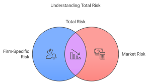
In portfolio management, understanding the types of risk is essential for making informed investment decisions. We can categorize risk into three main types:

1. 1. 1. Firm-Specific (Diversifiable) Risk: Risk factors unique to an individual company or industry that can be reduced or eliminated through diversification.
      2. Market (Non-Diversifiable) Risk: Risks that impact the entire market and cannot be mitigated by holding a diversified portfolio.
      3. Total Risk: The combination of both firm-specific and market risk.

This section will explore these risk categories in detail and explain how they affect investment decisions and portfolio construction.

8.5.2 Key Topics:

1. Firm-Specific (Diversifiable) Risk:

• • Definition: Firm-specific risk, also known as diversifiable or idiosyncratic risk, is associated with events or factors that affect only one company or a specific industry. These are risks that do not impact the entire market.
  • Examples of Firm-Specific Risks:
    • Product recalls due to quality issues
    • Changes in company leadership or strategic direction
    • Regulatory fines or legal issues
  • Why It’s Diversifiable: By holding a broad portfolio of stocks from various industries, investors can mitigate the impact of any single firm’s adverse event. The positive and negative performance of different firms tends to offset each other, reducing overall exposure to firm-specific risk.

Example: Suppose a pharmaceutical company faces a lawsuit over a product defect, causing a significant drop in its stock price. If an investor holds only this company’s stock, the loss is considerable. However, if the investor holds stocks across multiple sectors, the impact is minimized as other stocks in the portfolio may not be affected by the lawsuit.

2. Market (Non-Diversifiable) Risk:

• • Definition: Market risk, also known as systematic or non-diversifiable risk, is the risk that affects the entire market or economy. These risks cannot be reduced by diversification since they impact all securities to some extent.
  • Examples of Market Risks:
    • Economic downturns: A recession can reduce consumer spending, impacting companies across sectors.
    • Inflation and interest rate changes: Rising inflation or interest rates can increase borrowing costs and reduce profit margins.
    • Political or global events: Events such as elections, wars, or global pandemics can disrupt markets and lead to broad declines in stock prices.
  • Why It’s Non-Diversifiable: Because these risks impact the entire market, holding a diversified portfolio does not eliminate exposure to them. However, investors can manage market risk by considering asset classes with different risk levels, such as bonds, or by hedging.

Example: During the global financial crisis of 2008, almost all sectors and stocks experienced losses, regardless of the specific industry. This is an example of market risk, where diversification within stocks could not shield portfolios from the economic downturn’s effects.

3. Total Risk: Combining Firm-Specific and Market Risk

• • Definition: Total risk is the sum of firm-specific risk and market risk. It represents the overall variability in returns that an investor in a particular security or portfolio might experience.
  • Importance for Investors: Understanding total risk helps investors make better portfolio decisions by evaluating both the diversifiable and non-diversifiable risks they are exposed to. While diversification can reduce firm-specific risk, market risk will always remain as part of the total risk.
  • Using Total Risk in Portfolio Selection: Investors with high risk tolerance may choose portfolios with higher total risk to seek greater returns, while risk-averse investors may prefer lower total risk portfolios, even if the expected returns are lower.

Practical Application:

When building a portfolio, an investor aims to diversify away as much firm-specific risk as possible by holding a mix of assets from various industries. However, market risk remains, so understanding one’s tolerance for market swings is essential for setting realistic investment goals.

This concludes the discussion on types of risk in portfolios. In the next section, we’ll introduce Beta and Market Risk Measurement to quantify market risk for individual securities and examine its implications for portfolio management.

8.6 Understanding and Measuring Market Risk with Beta

8.6.1 Concept Overview:

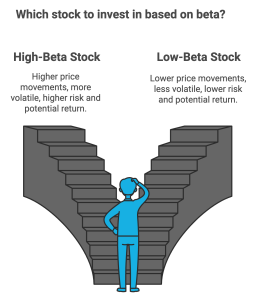
Beta (β) is a critical measure in finance that assesses a stock’s sensitivity to market movements. It quantifies market risk by evaluating how much a stock’s return is expected to change in response to fluctuations in the broader market. High-beta stocks are more volatile, often offering higher potential returns at increased risk. Conversely, low-beta stocks exhibit lower volatility, appealing to risk-averse investors.

8.6.2 Key Topics:

1. Definition and Calculation of Beta

What Beta Measures:

Beta reflects a stock’s relative risk compared to the overall market:

• • • A beta greater than 1 indicates the stock is more volatile than the market.
    • A beta less than 1 suggests the stock is less volatile.
    • A beta of 1 means the stock moves in line with the market.

Calculation of Beta:

Beta is calculated using the formula:

[latex]\beta = \frac{\text{Covariance of stock{\prime}s returns with the market}}{\text{Variance of the market{\prime}s returns}}[/latex]

The result quantifies how closely a stock’s returns correlate with the market.

Practical Calculation Example:

Suppose a stock has a beta of 1.5.

• • If the market rises or falls by 1%, the stock is expected to increase or decrease by 1.5%, making it more volatile than the market.

2. Interpretation of Beta Values:

• • Beta > 1: Stocks with a beta greater than 1 are more sensitive to market movements. They are likely to experience greater gains during market upturns and steeper losses during downturns. Examples include high-growth tech companies and cyclical industries.
  • Beta < 1: Stocks with a beta less than 1 are less sensitive to market changes, providing more stability but potentially lower returns. Examples include utility and consumer staple companies, which tend to have consistent demand.
  • Beta = 1: A beta of 1 suggests that the stock moves with the market, neither more volatile nor more stable. Index funds or ETFs that track the broader market typically have a beta of 1.

Example of Beta Values in Practice:

• • High Beta Stock: Tesla (historically) has had a beta greater than 1, indicating its stock price is more volatile than the market. Investors in high-beta stocks like Tesla are willing to accept higher risk in exchange for potentially higher returns.
  • Low Beta Stock: Johnson & Johnson, with a beta less than 1, tends to have a steadier stock price, appealing to more risk-averse investors.

3. Importance of Beta in Portfolio Management:

• • Portfolio Construction: Investors can use beta to manage portfolio risk. Combining high-beta and low-beta stocks allows for a diversified risk profile. For example, an investor might balance a high-beta technology stock with a low-beta consumer staples stock to create a more stable portfolio.
  • Risk Adjustment: Beta helps investors determine whether a stock fits their risk tolerance. Risk-averse investors may prefer stocks with lower beta values, while risk-tolerant investors might look for stocks with higher beta values.

4. Limitations of Beta as a Risk Measure:

• • Historical Nature: Beta is typically calculated using historical data, which may not predict future performance accurately.
  • Doesn’t Capture All Risks: Beta only measures market risk and does not account for firm-specific risks, economic changes, or industry shifts.
  • Non-Linear Behavior: During extreme market conditions, beta may not accurately represent a stock’s behavior, as some stocks may react unpredictably during economic crises.

Practical Application:

When managing a portfolio, beta is essential for understanding market risk exposure. Investors can adjust their portfolio’s average beta to align with their risk tolerance and financial goals, achieving a balance between risk and expected return.

In the next section, we will explore the Capital Asset Pricing Model (CAPM) and the Security Market Line (SML), which build on beta to establish a theoretical relationship between risk and expected return.

8.7 Capital Asset Pricing Model (CAPM) and the Security Market Line (SML)

8.7.1 Concept Overview:

The Capital Asset Pricing Model (CAPM) is a cornerstone in finance for understanding the relationship between risk and return. It proposes that investors should be compensated for two main components: the time value of money (represented by the risk-free rate) and the risk premium (based on market risk and the investment’s beta). This framework provides a way to calculate the expected return of an asset as a function of its systematic risk.

The Security Market Line (SML) visually represents the CAPM model, plotting the expected return of assets against their beta. It serves as a tool to assess whether an asset is fairly valued based on its risk-return tradeoff.

8.7.2 Key Topics:

1. The Formula and Components of CAPM:

• • The Formula and Components of CAPM:

The CAPM formula is:

[latex]\text{Expected Return } (k) = k_{\text{RF}} + \beta \times (k_{\text{M}} - k_{\text{RF}})[/latex]

Where:

• • [latex]k_{\text{RF}}[/latex] : Risk-Free Rate, typically the return on government bonds (e.g., 10-year U.S. Treasury bonds).
  • [latex]\beta[/latex] : Beta of the asset, indicating its sensitivity to market movements.
  • [latex]k_{\text{M}} - k_{\text{RF}}[/latex] : Market Risk Premium, the additional return expected from a diversified market portfolio over the risk-free rate.

Example Calculation:

• • Suppose:
    • Beta ( \beta ) = 1.5
    • Risk-Free Rate ( [latex]k_{\text{RF}}[/latex] ) = 3%
    • Market Expected Return ( [latex]k_{\text{M}}[/latex] ) = 10%

[latex]\text{Expected Return } = 3\% + 1.5 \times (10\% - 3\%) = 13.5\%[/latex]

This means the required return for this investment is 13.5%, given its higher exposure to market risk.

2. Understanding the Security Market Line (SML):

The SML is a graphical representation of the CAPM equation:

• • X-axis: Beta (Systematic Risk)
  • Y-axis: Expected Return

The SML’s slope represents the market risk premium, and its intercept is the risk-free rate.

• • Above the Line: Assets plotted above the SML offer higher returns than expected for their risk level and may be undervalued.
  • Below the Line: Assets below the SML offer lower returns for their risk level and may be overvalued.

3. Practical Implications of CAPM and SML:

• • Evaluating Stocks and Portfolios: CAPM helps investors decide if a stock or portfolio is attractive based on its risk-adjusted return. For example, a stock with a higher-than-expected return relative to its beta could be seen as undervalued.
  • Setting Investment Hurdle Rates: Companies often use CAPM to set minimum acceptable rates of return for projects, ensuring they’re compensated for the risk they take on.

4. Assumptions and Limitations of CAPM and SML:

• • Assumptions:
    • All investors have the same expectations about future returns and risks.
    • Markets are efficient, meaning prices reflect all available information.
    • Risk is adequately captured by beta, ignoring unsystematic risk.
  • Limitations:
    • Historical betas may not predict future volatility accurately.
    • Other factors, such as company size or momentum, may influence returns.
    • Assumes a single risk-free rate, which may not be realistic for international or multi-currency investments.

Real-World Relevance:

CAPM remains a widely used model in finance for evaluating assets and portfolio management, though it works best when combined with other tools. Understanding its assumptions and limitations helps investors apply it effectively.

This introduction lays the groundwork for CAPM’s practical application, which will be further discussed in later Chapter, focusing on the cost of equity and portfolio optimization.