11 Chapter 11 – Introduction of Capital Budgeting
Learning Objectives
- Identify the types of cash flows needed in the capital budgeting process.
- Forecast incremental earnings in a pro forma earnings statement for a project.
- Convert forecasted earnings to free cash flows and compute a project’s NPV.
- Recognize common pitfalls that arise in identifying a project’s incremental free cash flows.
- Assess the sensitivity of a project’s NPV to changes in assumptions.
- Identify the most common options available to managers in projects and understand why these options can be valuable.
11.1 The Capital Budgeting Process
Capital budgeting is a structured approach that companies use to evaluate long-term investment decisions. This process ensures resources are allocated effectively, minimizing risks and maximizing returns. Whether considering launching a new product, acquiring a competitor, or expanding into a new market, the capital budgeting process is essential for making informed financial decisions.
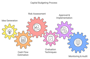
11.1.1 Key Steps in the Capital Budgeting Process
1. Idea Generation and Screening
-
- Firms generate project ideas from various sources, such as employee suggestions, market research, or technological advancements.
- These ideas are screened for feasibility, alignment with corporate goals, and resource availability.
2. Estimating Incremental Cash Flows
-
- Evaluate the additional cash inflows and outflows a project generates, excluding unrelated or sunk costs.
- Focus on the net effect the project has on the firm’s overall cash flow.
3. Assessing Risks
-
- Identify potential risks, such as market competition, regulatory changes, or cost overruns, that could affect the project’s performance.
- Apply risk analysis tools, like sensitivity analysis or scenario planning, to understand possible outcomes.
4. Selecting Evaluation Techniques
-
- Use financial metrics like Net Present Value (NPV), Internal Rate of Return (IRR), and Payback Period to assess the project’s financial viability.
- NPV is often favored for its ability to consider the time value of money and absolute value creation.
5. Approval and Implementation
-
- Present the evaluated project to decision-makers, like executives or the board of directors, for approval.
- If approved, allocate resources, create a timeline, and implement the project with ongoing oversight.
6. Monitoring and Post-Audit
-
- After project implementation, compare actual results with initial forecasts to evaluate performance.
- Use insights gained to refine future capital budgeting decisions.
11.1.2 Why the Capital Budgeting Process Matters
Capital budgeting aligns projects with a firm’s long-term goals, ensuring efficient use of limited resources. By rigorously evaluating potential investments, companies can:
-
- Increase shareholder value.
- Reduce financial risks.
- Adapt to changing market conditions.
Example of Capital Budgeting in Action
Consider a retail company, ABC Stores, evaluating the feasibility of opening a new branch.
-
- Estimated Cash Flows: Additional revenue from the branch is projected to be $1 million annually, with operational costs of $600,000.
- Initial Investment: $1.5 million for building and equipment.
- Evaluation: Using NPV at a discount rate of 8%, the firm estimates an NPV of $500,000, indicating a profitable investment.
By following the capital budgeting process, ABC Stores ensures resources are directed toward ventures with high potential returns, minimizing wasted capital on unprofitable initiatives.
11.2 Forecasting Incremental Earnings
Accurate forecasting of incremental earnings is a cornerstone of the capital budgeting process. Incremental earnings represent the additional net income a project generates, excluding sunk costs or unrelated revenues. By understanding the distinctions between operating expenses and capital expenditures, estimating revenues and costs, accounting for taxes, and creating comprehensive forecasts, firms can make well-informed investment decisions.
11.2.1 Operating Expenses Versus Capital Expenditures
When evaluating a project’s financial impact, it is essential to distinguish between operating expenses and capital expenditures, as they affect financial statements differently.
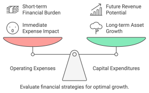 1. Operating Expenses:
-
- These are ongoing costs incurred to run the business, such as salaries, rent, and utilities.
- Operating expenses are fully deducted from revenues in the year they are incurred.
2. Capital Expenditures:
-
- These involve investments in long-term assets like equipment or buildings.
- Instead of being expensed immediately, capital expenditures are depreciated over the asset’s useful life, affecting earnings incrementally.
Example: Capital Expenditures vs. Operating Expenses
A company installs a new production line for $500,000 (capital expenditure) with annual maintenance costs of $20,000 (operating expense). The initial investment is depreciated over 10 years, contributing $50,000 annually to expenses.
11.2.2 Incremental Revenue and Cost Estimates
Identifying revenues and costs directly attributable to a project is vital for accurate forecasting.
1. Incremental Revenue
-
- Additional sales directly resulting from the project.
- Consider market demand, competition, and pricing strategies.
2. Incremental Costs
-
- Direct costs like materials and labor.
- Indirect costs such as overhead allocation.
Example: Estimating Incremental Revenue and Costs
A retail chain opens a new store projected to generate $1.2 million in annual sales, with operating costs of $800,000. Incremental revenue is $1.2 million, and incremental costs are $800,000, leaving incremental operating income of $400,000.
11.2.3 Taxes and Depreciation
Taxes significantly affect incremental earnings and must be accounted for. Depreciation, while non-cash, influences taxable income and reduces tax liability.
1. Taxable Income:
-
- Incremental operating income minus depreciation and other deductible expenses.
2. Tax Rate Application:
-
- Apply the corporate tax rate to calculate tax expense.
Example: Tax Impact on Incremental Earnings
Using the previous example:
- Operating income: $400,000
- Depreciation (capital expenditure): $50,000
- Taxable income: $400,000 - $50,000 = $350,000
- Taxes (at 30%): $350,000 × 0.30 = $105,000
- Incremental after-tax earnings: $400,000 - $105,000 = $295,000
11.2.4 Incremental Earnings Forecast
Combine all elements—incremental revenue, costs, capital expenditures, depreciation, and taxes—into a comprehensive incremental earnings forecast.
Example: Creating an Incremental Earnings Forecast
A manufacturing firm is evaluating a new machine costing $1,000,000 with a 5-year lifespan. The machine is expected to generate annual revenue of $600,000 and operating costs of $300,000.
Steps:
1. Calculate Annual Depreciation:
[latex]\text{Depreciation} = \frac{\text{Capital Expenditure}}{\text{Useful Life}} = \frac{1,000,000}{5} = 200,000[/latex]
2. Estimate Taxable Income:
[latex]\text{Taxable Income} = \text{Incremental Revenue} - \text{Incremental Costs} - \text{Depreciation}[/latex]
[latex]= 600,000 - 300,000 - 200,000 = 100,000[/latex]
3. Calculate Taxes:
[latex]\text{Taxes} = 100,000 \times 0.30 = 30,000[/latex]
4. Determine After-Tax Earnings:
[latex]\text{After-Tax Earnings} = 100,000 - 30,000 = 70,000[/latex]
11.3 Determining Incremental Free Cash Flow
Free Cash Flow (FCF) is a fundamental measure in capital budgeting. It represents the actual cash available to the firm after accounting for operating expenses, taxes, capital expenditures, and changes in working capital. Understanding how to calculate incremental FCF is essential for evaluating a project’s viability and determining its Net Present Value (NPV).
11.3.1 Converting from Earnings to Free Cash Flow
While incremental earnings are a starting point, they do not reflect the actual cash flow because of non-cash charges like depreciation and changes in working capital. FCF is computed by adjusting incremental earnings to account for these factors.
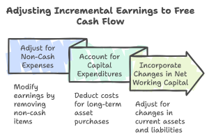
1. Adjust for Non-Cash Expenses:
-
- Add back depreciation and other non-cash charges since they don’t involve actual cash outflow.
2. Account for Capital Expenditures:
-
- Subtract cash spent on capital investments needed to sustain or grow the project.
3. Incorporate Changes in Net Working Capital (NWC):
-
- Adjust for increases or decreases in NWC, which reflect short-term cash tied up in operations.
Formula: Free Cash Flow
[latex]\text{FCF} = \text{Incremental Earnings} + \text{Depreciation} - \text{Capital Expenditures} - \Delta \text{NWC}[/latex]
Where:
-
- Depreciation: Non-cash expense added back to earnings.
- Capital Expenditures: Cash outflows for long-term investments.
- NWC: Changes in net working capital, such as inventory or receivables.
Example: Calculating FCF from Earnings
A project generates $500,000 in incremental earnings annually, with $150,000 in depreciation, $200,000 in capital expenditures, and an increase in NWC of $50,000.
[latex]\text{FCF} = 500,000 + 150,000 - 200,000 - 50,000 = 400,000[/latex]
The project’s annual free cash flow is $400,000.
11.3.2 Calculating Free Cash Flow Directly
Instead of starting from incremental earnings, FCF can be computed directly by evaluating cash inflows and outflows.
Formula: Direct FCF Calculation
[latex]\text{FCF} = \text{Cash Revenue} - \text{Cash Costs} - \text{Taxes} - \text{Capital Expenditures} - \Delta \text{NWC}[/latex]
Example: Direct Calculation
A project produces $800,000 in cash revenue, incurs $400,000 in cash costs, requires $250,000 in capital expenditures, and causes a $60,000 increase in NWC. Taxes on operating income are 30%.
1. Operating Income:
[latex]800,000 - 400,000 = 400,000[/latex]
2. Taxes:
[latex]400,000 \times 0.30 = 120,000[/latex]
3.FCF:
[latex]800,000 - 400,000 - 120,000 - 250,000 - 60,000 = 430,000[/latex]
The FCF for this project is $430,000 per year.
11.3.3 Calculating the NPV
Net Present Value (NPV) measures the profitability of a project by discounting future cash flows to their present value and comparing them to the initial investment.
Formula: NPV
$$\text{NPV} = \sum_{t=1}^{n} \frac{\text{FCF}_t}{(1 + r)^t} - \text{Initial Investment}$$
Where:
-
- \[
\text{FCF}_t = \text{Free Cash Flow in year } t
\] - \[
r = \text{Discount rate (usually WACC)}
\] - \[
n = \text{Number of years}
\]
- \[
Example: Calculating NPV
A project requires an initial investment of $1 million and is expected to generate $300,000 in annual FCF for five years. The discount rate is 8%.
1. Present Value of Cash Flows
$$\text{PV} = \frac{300,000}{(1 + 0.08)^1} + \frac{300,000}{(1 + 0.08)^2} + \cdots + \frac{300,000}{(1 + 0.08)^5}$$
Using a financial calculator or Excel, the total PV is approximately $1,197,000.
2. NPV Calculation
[latex]\text{NPV} = 1,197,000 - 1,000,000 = 197,000[/latex]
The project’s NPV is $197,000, indicating a profitable investment.
Key Takeaway
Determining FCF and NPV ensures that decision-makers can objectively evaluate a project’s financial feasibility. By converting incremental earnings to cash flow, accounting for all inflows and outflows, and using discounted cash flow analysis, firms can identify projects that maximize shareholder value.
11.4 Other Effects on Incremental Free Cash Flows
When evaluating incremental free cash flows, it’s crucial to consider factors beyond direct revenues and costs. These additional elements, such as opportunity costs, project externalities, sunk costs, and adjustments to free cash flow, can significantly influence a project’s valuation. By accounting for these effects, firms can make more accurate financial assessments.
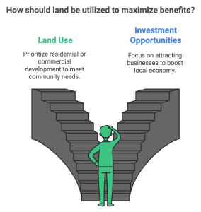
11.4.1 Opportunity Costs
Definition
Opportunity cost refers to the value of the next-best alternative that is sacrificed when resources are allocated to a specific project. Failing to account for opportunity costs can lead to an overestimation of a project’s value.
Why It Matters
Opportunity costs ensure that resources like capital, land, or equipment are allocated to their most productive use. Incorporating opportunity costs into analysis helps avoid missed opportunities elsewhere.
Example: Land Use Opportunity Cost
A company owns a plot of land purchased for $1 million five years ago. Its market value today is $1.5 million, and it could be sold or leased for alternative uses. If the company uses the land for a new project, the opportunity cost is $1.5 million, which must be included in the project evaluation.
11.4.2 Project Externalities
Definition
Project externalities are indirect effects a new project has on other parts of the business. These can either enhance (synergies) or reduce (cannibalization) overall profitability.
-
- Synergies: Positive externalities that benefit other areas of the business, such as increased brand recognition or cross-selling opportunities.
- Cannibalization: Negative externalities where the new project reduces revenue or profitability from existing products or services.
Example: Product Cannibalization
A car manufacturer launches a new electric vehicle model that generates $10 million in annual revenue. However, $3 million of this comes at the expense of reduced sales from its existing hybrid model. The net incremental revenue is $7 million after accounting for cannibalization.
11.4.3 Sunk Costs
Definition
Sunk costs are expenses already incurred and cannot be recovered. They are irrelevant for future decision-making, as they should not influence whether to proceed with a project.
Why Ignore Sunk Costs?
Decisions should focus on incremental costs and benefits rather than past expenditures.
Example: Ignoring Sunk Costs
A company spends $200,000 on market research for a new product. Later, the company decides not to proceed with the product. The $200,000 is a sunk cost and should not influence decisions about alternate projects or new product ideas.
This approach prevents firms from making biased decisions based on past expenditures rather than current opportunities.
11.4.4 Adjusting Free Cash Flow
Free cash flow calculations must reflect realistic adjustments for changes in working capital, taxes, and unforeseen costs. Accurate adjustments ensure that FCF aligns with real-world operations.
1. Working Capital Adjustments
Cash tied up in inventory or receivables reduces FCF, while a reduction in working capital increases it.
2. Tax Effects
Proper tax adjustments ensure that net cash flow reflects actual after-tax income.
Example: Adjusting for Working Capital
A project requires an initial increase in inventory of $500,000. At the end of the project, $300,000 of this working capital is recovered. The adjustments are as follows:
-
- Year 0: Deduct $500,000 as an initial outflow.
- Final Year: Add back $300,000 as a recovered inflow.
11.4.5 Replacement Decisions
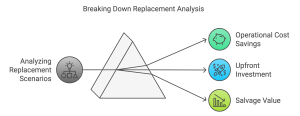
Definition
Replacement decisions involve evaluating whether replacing an existing asset with a new one offers a net benefit. The analysis considers the cost of the new asset, operational cost savings, and the salvage value of the old asset.
Steps in Replacement Decisions
-
- Evaluate operational cost savings from the new asset.
- Subtract the upfront investment in the replacement asset.
- Add the salvage value of the replaced asset.
Example: Equipment Replacement
A company is deciding whether to replace a machine. The current machine costs $50,000 annually in operations and has no resale value. A new machine costs $200,000 but reduces operating costs to $20,000 annually.
1. Annual Savings:
[latex]\text{Savings Per Year} = 50,000 - 20,000 = 30,000[/latex]
2. Present Value of Savings (5 years, 8% discount rate):
$$\text{PV} = 30,000 \left( \frac{1 - (1 + 0.08)^{-5}}{0.08} \right) \approx 120,600$$
3. Net Impact:
[latex]\text{Net Impact} = 120,600 - 200,000 = -79,400[/latex]
The analysis shows that replacing the machine is not cost-effective under the given assumptions.
Key Takeaway
Considering additional effects on incremental free cash flows, such as opportunity costs, externalities, sunk costs, and working capital adjustments, ensures a more accurate and comprehensive project evaluation. These elements help firms avoid pitfalls and make more informed decisions.
11.5 Analyzing the Project
Evaluating a project’s financial and operational viability involves testing its robustness under various conditions. This section focuses on techniques like sensitivity analysis, break-even analysis, and scenario analysis to identify key variables affecting project outcomes, assess risks, and understand the potential range of results.
11.5.1 Sensitivity Analysis
Definition
Sensitivity analysis examines how changes in a single variable—such as sales volume, cost of capital, or operating costs—impact key project metrics like Net Present Value (NPV) or Internal Rate of Return (IRR).
Why It’s Useful
It helps identify critical variables and assess the project’s resilience to changes in assumptions.
Steps for Conducting Sensitivity Analysis
-
- Identify key variables (e.g., revenue growth, operating costs, discount rate).
- Change one variable at a time, keeping all others constant.
- Recalculate the project’s NPV or IRR for each change.
- Plot results to visualize sensitivity.
Example: Sensitivity of NPV to Revenue Growth
A project’s base case assumes 10% annual revenue growth, leading to an NPV of $200,000. The analysis tests growth rates of 8%, 12%, and 15%.
-
- At 8% Growth: NPV drops to $150,000.
- At 12% Growth: NPV rises to $250,000.
- At 15% Growth: NPV jumps to $300,000.
This analysis highlights the project’s heavy reliance on revenue growth.
11.5.2 Break-Even Analysis
Break-even analysis identifies the point where the project generates enough cash flow to cover its costs, resulting in a zero NPV. It’s particularly useful for evaluating the feasibility of a project under varying assumptions.
Formula: Break-Even Sales Volume
[latex]\text{Break-Even Sales Volume} = \frac{\text{Fixed Costs}}{\text{Price per Unit} - \text{Variable Cost per Unit}}[/latex]
Example: Calculating Break-Even Sales Volume
A project has:
-
- Fixed Costs: $500,000
- Price per Unit: $50
- Variable Cost per Unit: $30
Break-Even Sales Volume:
[latex]\text{Break-Even Sales Volume} = \frac{500,000}{50 - 30} = 25,000 \text{ units}[/latex]
The project needs to sell 25,000 units to break even.
11.5.3 Scenario Analysis
Definition
Scenario analysis evaluates how a combination of changes in multiple variables impacts project outcomes. Unlike sensitivity analysis, which tests one variable at a time, scenario analysis considers multiple factors simultaneously to provide a range of potential results.
Key Scenarios
-
- Best Case: Assumes favorable conditions, such as higher revenue growth or lower costs.
- Worst Case: Assumes unfavorable conditions, such as declining demand or rising costs.
- Base Case: Assumes the most likely conditions based on current forecasts.
Example: Analyzing Three Scenarios
A project with a base-case NPV of $200,000 is evaluated under varying conditions:
1. Best Case:
-
- Revenue grows by 15% annually.
- Costs decrease by 5%.
- NPV = $350,000.
2. Worst Case:
-
- Revenue grows by 5% annually.
- Costs increase by 10%.
- NPV = $50,000.
3. Base Case:
-
- Revenue grows by 10% annually.
- Costs remain stable.
- NPV = $200,000.
Scenario analysis provides insight into the range of possible outcomes, helping managers prepare for uncertainties.
Key Takeaway
Project analysis techniques like sensitivity analysis, break-even analysis, and scenario analysis allow managers to identify critical variables, evaluate risks, and understand the range of possible outcomes. By integrating these tools, firms can make more informed decisions, ensuring robust project evaluations.
11.6 Real Options in Capital Budgeting
Capital budgeting traditionally assumes static decisions, but real-world projects often evolve based on new information. Real options in capital budgeting provide managers with flexibility, allowing them to adapt investment decisions to changing circumstances. These options add value by enabling firms to delay, expand, or abandon projects as conditions evolve.
11.6.1 Option to Delay
Definition
The option to delay allows firms to postpone an investment decision until more information is available, reducing uncertainty and risk. This is particularly valuable in volatile markets.
When to Use
-
- High market uncertainty.
- Large upfront costs with uncertain returns.
- New product launches where market acceptance is unclear.
Example: Delaying a New Product Launch
A company plans to invest $10 million in launching a new product. However, demand is uncertain due to economic instability. By delaying the project by a year, the company can gather market data, reducing the risk of launching into a weak market.
If the market rebounds, the project moves forward; otherwise, the company avoids the potential loss.
11.6.2 Option to Expand
Definition
The option to expand gives firms the ability to scale up a project if it performs better than expected. This flexibility enhances the project’s overall value by capturing upside potential.
When to Use
-
- High-growth markets with strong demand potential.
- Initial projects designed with modular or scalable capacity.
Example: Expanding a Manufacturing Facility
A company invests $10 million in a facility with a capacity of 10,000 units but includes an option to double capacity for an additional $6 million. If demand exceeds expectations, the firm exercises the expansion option, increasing capacity to 20,000 units and capitalizing on market opportunities.
11.6.3 Option to Abandon
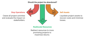
Definition
The option to abandon allows firms to terminate a project if it becomes unprofitable or unsustainable, minimizing further losses.
When to Use
-
- Declining market conditions or regulatory changes.
- High initial uncertainty about the project’s success.
Example: Abandoning a Retail Expansion
A retail chain opens a pilot store in a new region, investing $1 million. After two years, sales are significantly below expectations, and the local market shows limited growth potential. The company decides to abandon the expansion, selling the store and reallocating resources to more profitable regions.
This decision minimizes losses and prevents further capital from being tied up in an unviable project.
Strategic Value of Real Options
Real options create strategic value by:
-
- Enhancing Flexibility: Adapting to uncertainties ensures that firms can respond dynamically to market conditions.
- Reducing Downside Risk: Options like abandonment limit losses on failing projects.
- Capturing Upside Potential: Expansion options allow firms to maximize gains in favorable conditions.
Key Takeaways
-
- Real Options Provide Flexibility: Firms can delay, expand, or abandon projects, adapting decisions to changing circumstances.
- Option to Delay: Delaying projects can reduce uncertainty, especially in volatile markets.
- Option to Expand: Expansion options enable firms to capitalize on favorable outcomes, increasing project value.
- Option to Abandon: Abandoning unviable projects minimizes losses and reallocates resources to better opportunities.
- Strategic Use: Real options improve decision-making, ensuring projects remain resilient to uncertainty and market dynamics.
Key Takeaways
- Capital Budgeting Guides Long-Term Decisions: It ensures investments align with strategic goals and create value.
- Free Cash Flow is Key: Projects are evaluated by converting earnings to free cash flow, capturing actual cash availability.
- NPV as a Decision Metric: Positive NPV indicates a project is likely to add value to the firm.
- Sunk Costs Don’t Matter: Focus only on future costs and benefits, ignoring past expenditures.
- Real Options Provide Flexibility: Options to delay, expand, or abandon projects help adapt to changing conditions.
- Risk Analysis is Crucial: Sensitivity and scenario analyses test project outcomes under varying assumptions.
Exercises
Conceptual Questions
-
- What is capital budgeting, and why is it important for making long-term investment decisions?
- Differentiate between incremental cash flows and sunk costs. Provide an example of each.
- Why are opportunity costs considered in capital budgeting? Explain with an example.
- What is NPV, and how does it differ from other evaluation metrics like IRR and Payback Period?
- How do real options such as the option to delay, expand, or abandon a project enhance decision-making in capital budgeting?
Short Calculations
1. Depreciation Calculation
A project requires purchasing machinery for $600,000 with a useful life of 8 years. Calculate the annual depreciation expense.
2. Free Cash Flow Calculation
A project generates $300,000 in incremental earnings annually, with $80,000 in depreciation, $100,000 in capital expenditures, and a $40,000 increase in working capital. Calculate the annual free cash flow (FCF).
3. Net Present Value Calculation
A project requires an initial investment of $1.2 million and is expected to generate annual free cash flows of $400,000 for 4 years. The discount rate is 10%. Calculate the Net Present Value (NPV).
Scenario-Based Problems
1. Break-Even Analysis
A project has fixed costs of $500,000, a selling price of $60 per unit, and variable costs of $35 per unit. Calculate the break-even sales volume.
2. Sensitivity Analysis
A project assumes 12% annual revenue growth, resulting in an NPV of $400,000. Perform a sensitivity analysis by calculating the NPV if revenue growth drops to 8% or increases to 15%.
3. Real Options Challenge
A firm has the option to delay a $3 million investment for one year to gather more market data. Discuss under what circumstances delaying the project might add value and what factors would influence the decision.
Interactive Challenge
1. Assessing Project Viability
A company is evaluating a new project requiring a $2 million investment. The project is expected to generate annual free cash flows of $600,000 for five years. The discount rate is 8%.
Task: Determine whether the project is viable by calculating the NPV.
Hint: Use the formula for NPV and a financial calculator or Excel if needed.
2. Real Options: Delay vs. Immediate Investment
A firm is considering a $5 million project but is uncertain about market conditions. The firm can delay the project by one year to gain more information, incurring a $100,000 holding cost. If the project is delayed, new market data might suggest an increase in returns, improving free cash flows by 20%.
Task: Compare the benefits of delaying versus investing immediately.
Hint: Calculate the potential additional NPV from delaying the project.
3. Scenario Analysis for a Manufacturing Facility
A manufacturing company plans to invest in a new production facility. The base case assumes $1.5 million in annual revenue growth, $800,000 in costs, and an NPV of $250,000. Under the best-case scenario, revenue grows to $2 million, while under the worst case, revenue falls to $1 million.
Task:
-
- Calculate the NPV for the best-case and worst-case scenarios.
- Determine whether the project remains viable under these conditions.
4. Identify Key Variables in Sensitivity Analysis
A retail firm is exploring a new store location with an initial investment of $1 million. The NPV is most sensitive to changes in sales volume, which directly impacts revenue, and rent costs, which affect fixed expenses.
Task:
-
- Identify how a 10% increase or decrease in sales volume impacts the NPV.
- Explore how a 15% rise in rent costs changes the project’s viability.
- Recommend strategies to mitigate risks related to these variables.
