4 Chapter 4 – Interest Rate

4.1 Interest Rate Quotes and Adjustments

4.1.1 Introduction to Interest Rates

Definition and Importance

Interest rates represent the cost of borrowing money or the return on invested capital. This cost or return is often expressed as a percentage of the principal amount on an annual basis. Interest rates are central to financial decision-making, influencing everything from personal loans and savings accounts to corporate investments and government bonds. By understanding interest rates, borrowers and investors can make informed choices about loans, investments, and savings.

Fundamental Concepts:

• • Principal: The original amount of money borrowed or invested.
  • Compounding: The process by which interest is calculated on both the initial principal and the accumulated interest from previous periods.
  • Time Value of Money (TVM): The foundational idea that a dollar today is worth more than a dollar in the future due to its earning potential.

4.1.2 Key Types of Interest Rates

Annual Percentage Rate (APR):

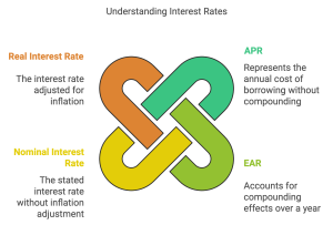
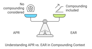
• • Definition: APR is the nominal or stated interest rate expressed on an annual basis, commonly used for loans and credit products. APR does not account for the effects of compounding within the year.
  • Application: APR is useful for comparing credit products that compound interest at the same frequency, such as monthly or quarterly.
  • Example: Suppose you take a loan with a 12% APR compounded monthly. This means each month, interest is calculated at 1% (12% ÷ 12 months).
  • Limitations: Since APR does not factor in the effects of compounding, it can understate the true cost of a loan if compounding occurs more than once per year.

Effective Annual Rate (EAR):

• • Definition: EAR, also called the annual equivalent rate, incorporates the effects of compounding within the year, giving a more accurate representation of the true annual interest rate.
  • Formula:

[latex]\text{EAR} = \left(1 + \frac{\text{APR}}{n}\right)^n - 1[/latex]

where n is the number of compounding periods per year.

• • Example Calculation: For a 12% APR loan compounded monthly, the EAR calculation would be:

[latex]\text{EAR} = \left(1 + \frac{0.12}{12}\right)^{12} - 1 \approx 0.1268 \text{ or 12.68%}[/latex]

• • Practical Meaning: The EAR of 12.68% represents the actual annual cost of the loan when compounding is considered. This value is higher than the APR due to monthly compounding.

4.1.3 Adjusting Discount Rates for Different Time Periods

Importance of Adjusting Rates:

Financial scenarios often require calculations over different time periods, making it necessary to adjust interest rates for accurate present or future value calculations. Converting rates helps maintain consistency across different compounding frequencies.

Adjusting to Different Compounding Periods:

• • Monthly Rate: Divide the APR by 12 for monthly compounding.
  • Quarterly Rate: Divide the APR by 4 for quarterly compounding.
  • Example Calculation: For a 12% APR compounded monthly, the monthly rate would be:

[latex]\text{Monthly Rate} = \frac{12\%}{12} = 1\%[/latex]

Converting APR to Match Different Time Periods:

• • Converting Annual Rate to Semi-Annual: Suppose we have a 6% APR with semi-annual compounding. To calculate the effective rate for a 6-month period:

[latex]\text{Semi-Annual Rate} = \left(1 + \frac{0.06}{2}\right)^2 - 1[/latex]

• • Practical Tip: Adjusting rates ensures that cash flows are accurately compared, regardless of compounding frequency.

4.1.4 Practical Applications and Key Takeaways

Using APR and EAR:

• • APR is useful for straightforward comparisons when compounding frequencies are the same but does not account for the effects of compounding.
  • EAR provides a more accurate representation of the true annual cost or yield and is essential when compounding frequencies differ.

Compounding Frequency Matters:

• • The frequency of compounding significantly impacts the actual return on investments or the cost of loans over time.
  • Higher compounding frequencies result in a higher EAR for the same APR, emphasizing the importance of understanding how compounding affects financial outcomes.

Final Reminder on Calculations:

• • Always adjust APR for the correct compounding period when calculating future or present values to ensure consistency in financial analysis.
  • Use EAR to accurately compare loans or investments with different compounding intervals, as it accounts for the true cost or return over time.

4.2 Application – Discount Rates and Loans

4.2.1 Introduction to Loan Calculations

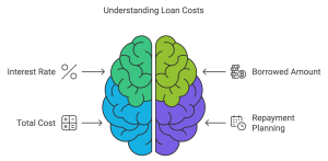
Loans are a critical component of personal and business finance, and understanding their structure helps borrowers make better financial decisions. Loan payments often involve both the repayment of principal (the amount borrowed) and interest (the cost of borrowing). The process of gradually repaying a loan over time through fixed payments is known as amortization.

Key Concepts:

• • Principal: The original amount borrowed.
  • Interest: The cost of borrowing, calculated as a percentage of the outstanding balance.
  • Amortization: The process of systematically reducing a loan balance over time through fixed payments.

4.2.2 Computing Loan Payments

Fixed-payment loans, such as mortgages or car loans, divide each payment into two parts: interest and principal repayment. As the loan progresses, the portion allocated to interest decreases, and the portion allocated to the principal increases.

Loan Payment Formula (for Fixed-Rate Loans):

The formula to calculate the monthly loan payment for a fixed-rate loan is:

$$\text{PMT} = \frac{P \times r}{1 – (1 + r)^{-n}}$$

Where:

• • PMT = Monthly payment
  • P = Principal (initial loan amount)
  • r = Monthly interest rate (annual rate divided by 12)
  • n = Total number of payments (loan term in years multiplied by 12)

4.2.3 Computing the Outstanding Loan Balance

The outstanding loan balance is the amount still owed at any point during the loan term. As monthly payments are made, the principal balance decreases, and each payment reduces the outstanding balance by a larger amount over time.

To calculate the outstanding balance after a certain number of payments, we can use a variation of the loan payment formula, focusing on the remaining payments.

Outstanding Balance Formula:

$$\text{Balance} = P \times \left( \frac{(1 + r)^n – (1 + r)^p}{(1 + r)^n – 1} \right)$$

Where:

• • Balance = Outstanding loan balance after p payments
  • P = Principal (initial loan amount)
  • r = Monthly interest rate
  • n = Total number of payments
  • p = Number of payments made so far

4.3: The Determinants of Interest Rates

Interest rates are influenced by various economic factors, including inflation, monetary policy, market conditions, and risk perceptions. Understanding these determinants is crucial for borrowers, investors, and businesses to make informed decisions about loans, savings, and investments.

4.3.1 Inflation and Real Versus Nominal Rates

Inflation Overview:

• • Inflation measures the general increase in prices over time, eroding the purchasing power of money.
  • Lenders require compensation for inflation, which is reflected in higher nominal interest rates.

Nominal vs. Real Interest Rates:

• • Nominal Interest Rate: The stated rate, including inflation expectations.
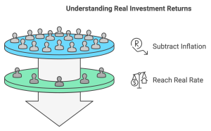
  • Real Interest Rate: The rate adjusted for inflation, reflecting true purchasing power.
  • Formula:

[latex]\text{Real Interest Rate} = \frac{1 + \text{Nominal Rate}}{1 + \text{Inflation Rate}} - 1[/latex]

Approximation for modest inflation:

[latex]\text{Real Rate} \approx \text{Nominal Rate} - \text{Inflation Rate}[/latex]

4.3.2 Investment and Interest Rate Policy

Concept Overview:

Interest rates are a powerful tool in influencing economic activity. For businesses and individuals, they dictate borrowing costs and potential returns on investments. Central banks, such as the U.S. Federal Reserve, adjust interest rates as part of their monetary policy to regulate inflation, promote economic growth, or cool down overheated markets.

Role of Central Banks:

• • Central banks like the Federal Reserve adjust interest rates through monetary policy to influence economic activity.
  • Lower rates stimulate borrowing and spending; higher rates control inflation by slowing economic growth.

4.3.3 The Yield Curve and Discount Rates

Concept Overview:

• • The yield curve plots interest rates for bonds of varying maturities.
  • A “normal” yield curve slopes upward, with long-term rates higher than short-term rates.

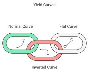
Types of Yield Curves:

1. 1. Normal Yield Curve: Long-term rates are higher than short-term rates, signaling economic growth expectations.
   2. Inverted Yield Curve: Short-term rates are higher than long-term rates, often a signal of an upcoming recession.
   3. Flat Yield Curve: Short- and long-term rates are similar, often indicating uncertainty in economic conditions.

Real-World Example: Interpreting an Inverted Yield Curve

An inverted yield curve has historically been a reliable predictor of recession. For example, in 2006, the U.S. yield curve inverted, and by late 2007, the economy entered the Great Recession. Financial institutions and investors watch yield curves closely as signals for economic forecasting.

4.3.5 Key Takeaways

1. 1. Inflation and Real Rates: Inflation affects the real return on investments. Nominal rates include inflation expectations, but real rates reflect true purchasing power.
   2. Interest Rate Policy and Investment: Central banks use interest rate adjustments to influence economic activity, with low rates spurring investment and high rates cooling spending.
   3. Yield Curve: The shape of the yield curve reflects economic expectations. An inverted yield curve, for example, can signal recession concerns.