Near the equator on a clear day at noon the solar radiation intensity will be about $1000\;\rm W/m^2$. If a solar panel was able to perfectly convert that light into electrical power, then a 1 square metre panel would provide 1000 W of electrical power under ideal conditions. Photovoltaic conversion is only about 20% efficient, limiting the output to about $200\;\rm W/m^2$ and with practical layout limitations a typical production panel of 2 square metres might yield 380 W.

At the equator on a clear day, facing the sun

Each solar panel contains many solar cells connected in series. Each cell can reach a potential of about 0.5 V, so the output of a typical 60 cell grid-tie panel would be about 30 volts of direct current (DC) in optimal operation. The best source of information about the performance of a particular panel is the manufacturer’s data sheet. For example the LG Electronics LG380N2T-A5 panels have 72 cells and at standard test conditions (STC) produce their maximum power of 380 W at 40.6 V with a current output of 9.37 A. In order to get this maximum performance, the load has to be just right.

Optimizing the load for maximum power output

Continuing with the LG panel at STC, the open circuit voltage will be 49 V if there is a very high resistance load connected and little or no current flowing. The resulting power to the load will be $P = VI \approx 0$. Similarly the short circuit current of 10.07 A at near 0 volts across a very low resistance load also yields no power. So let’s try a load composed of a 100 Ohm resistance, and estimate performance starting from the open circuit voltage. Note that Ohm’s Law ($V=IR$) is worth committing to memory even if you aren’t planning a career in Electrical Engineering.

\begin{equation}

I = \frac{V}{R} = \frac{49}{100} = 0.49{\;\rm A}\quad\quad P = VI = 49\times 0.49 = 24\;\rm W

\end{equation}

The voltage will drop a little once some current starts flowing, as shown on the characteristic curve, so we wouldn’t get quite all of that 24 W of power. Since we are at full sun on the equator for now, we will be looking at the red curve in the diagram.

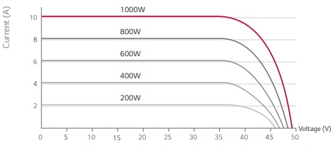
Clearly we would get even more power if we allowed more current to flow by reducing the load resistance, so let’s try 10 Ohms and adjust the voltage until we fall on the characteristic curve

\begin{equation}

I = \frac{V}{R} = \frac{49}{10} = 4.9{\;\rm A}\quad\quad P = VI = 49\times 4.9 = 240\;\rm W

\end{equation}

which is way closer to what we want, although at 5 A we will only have an output voltage of about 47 V from the panel, so it will be more like

\begin{equation}

I = \frac{V}{R} = \frac{47}{10} = 4.7{\;\rm A}\quad\quad P = VI = 47\times 4.7 = 221\;\rm W

\end{equation}

There’s no way to zero in on a closed form solution because we don’t have an analytical expression for the characteristic curve, so we iterate to get close. Let’s try again at 2 Ohms and we’ll find the current won’t go above 10.07, so the voltage drops to match

\begin{equation}

V = IR = 10.07\times 2 = 20{\;\rm V}\quad\quad P = VI = 20\times 10.07 = 201\;\rm W

\end{equation}

and we have even less power. If we keep on changing the load resistance to maximize the power output, we will eventually settle in at 9.37 A and 40.6 V, just under the maximum current output the panel can deliver. The corresponding load resistance will be

\begin{equation}

R = \frac{V}{I} = \frac{40.6}{9.37} = 4.33{\;\rm\Omega}\quad\quad P = VI = 40.6\times 9.37 = 380\;\rm W

\end{equation}

which is just fine except for two things: We will need to keep adjusting the resistor whenever the solar intensity changes due to angle or weather, or… and passing current through a resistor doesn’t do anything useful other than heat up the resistor. We need a way to operate this panel at that maximum power point while doing something useful like charging batteries.

Maximum Power Point Tracking (MPPT)

Whether or not we are on the equator and facing the sun, an MPPT charge controller will constantly scan the operating conditions of the panel for changes and adjust its DC:DC conversion system to take current from the panels at the maximum power point available and provide charging current to the batteries at the right DC voltage for best charging. Fortunately these controllers are available as existing products and we don’t need to design one from scratch. The MidNite Solar KID charge controller is an example.

Not facing the sun

If the panel is at an incidence angle of $\theta =90$ degrees, perpendicular to the sun’s rays, you will get the full intensity of the solar radiation. If the sun’s rays are striking the panel at a really small angle of incidence there will be significant reflection from the face of the panel, and the intensity will also be reduced based on the projected area so there will be little power produced. At reasonable angles you can get a good approximation by multiplying the intensity by the sine of the incidence angle $\theta$.

Latitude and weather and smog

Anything that reduces the solar intensity will also decrease the output of your solar panel proportionately. Light needs to pass through more atmosphere on a path to locations at higher latitudes, so the sun there is never as strong as the sun at the equator. Clouds block and scatter light so that the intensity is lower and it is more diffuse, coming from multiple directions. Smog or other particles in the air will have similar effects, reducing the actual power from the panel below the nameplate power at STC due to those combined effects, represented here by a transmission factor, $0<=f<=1$.

\begin{equation}

P_{actual} = fP_{STC} \sin\theta

\end{equation}

Practical Estimates from Historical Data

Given the complexities of determining $f$, the usual way to approach the problem is through either time histories or average values tabulated from measurements. For example, Natural Resources Canada (NRCan) reports that the “Mean daily global insolation” on a panel that is “South-facing tilt=lat+15°” for December in Kingston is 2.73 “kWh/m2 or full sun hours (h)” covering both atmospheric effects and incidence angle. We can use this information to predict that a typical December day in Kingston will produce the same amount of energy as we would get from 2.73 hours at STC. Our 380 W panel would produce an energy output of

\[2.73\times 380= 1037{\;\rm Wh}= 1.04{\;\rm kWh/day}\]

Keep in mind that’s an average day, with no guarantees we would get this much energy every day, or that we might not go for a week of really dreary weather, so predicting actual performance will have to consider day by day or even hour by hour time history data in a simulation.

The same NRCan dataset says we could get 13% more with two axis tracking, but that would add complex machinery and controls. If our targets are the best collection results in darkest December, then a panel aimed due south at an elevation angle of (44 + 15) = 59 degrees would be an easy compromise.

Getting the average 27 kWh/day we used in our condo would require 26 panels, costing more than \$12000 without factoring in the rest of the system. Making no allowance for interest, that would take eight and a half years just to pay off the panels, although we might also be able to sell some of our power through the Feed-In-Tariff (FIT) if we had a grid connection. Your solar system will probably require somewhere between the two panels of Signature and the twenty six that would be required for our condo.

This Jupyter Notebook (check the resources for software information) uses the pysolar library and python to calculate instantaneous solar intensity under a clear sky at different times of the year, and allows you to compare those results to some of the NRCan data. This CSV file contains an abbreviated subset of the NRCan data for Kingston and is loaded by the Jupyter Notebook, so save them both in the same folder.

The Historical Solar Data Notebook provides an example of some data from a Typical Meteorological Year (TMR), allowing us to see the variability between sunny and cloudy days. You will need the Toronto TMY CSV file to import into the notebook.

Other factors

PV panels age. They don’t perform as well when they are hot. There are energy conversion losses in every stage of the process. Panels may be covered with snow (although it will usually melt off pretty quickly) or partially shaded by obstructions. The more detailed the model you use, the closer you will get to the actual results, but what we have so far will provide a good basis for estimation of what’s possible.