Estimating a population mean (CI for 1 mean, sigma unknown)
More good stuff! We will need to know how to compute the margin of error, and then how to use that along with other pieces of information to compute or construct the confidence interval.
The Margin of Error for 1 Mean, σ Unknown:
The Confidence Interval for 1 Mean, σ Unknown:
| Basic Form | Inequalities | Interval Notation |
| [latex]\bar{x} \pm E[/latex] | [latex]\bar{x} - E \le \mu \le \bar{x} + E[/latex] | [latex](\bar{x} - E, \bar{x} + E)[/latex] |
What the different symbols mean:
[latex]n[/latex] is the sample size (number of people, items, etc… in the study)
[latex]\mu[/latex] is the population mean
[latex]\bar{x}[/latex] is the sample mean (also known as average)
[latex]s[/latex] is the sample standard deviation (sometimes this is given, sometimes we have to compute it)
[latex]E[/latex] is the margin of error
[latex]\alpha[/latex] is what is “left over” from the confidence level; we will look this up in the t-distribution table as an area in “two-tails”
[latex]df = n - 1[/latex] is the degrees of freedom; this will be used in conjunction with [latex]\alpha[/latex] in the t-distribution table
[latex]t_{\frac{\alpha}{2}}[/latex] is the critical value; this time we have to use the t-distribution table
Assumptions when estimating 1 Mean, σ Unknown:
- We have a simple random sample
- We have a normal distribution OR [latex]n\ge 30[/latex]
Steps to construct the Confidence Interval for 1 Mean, σ Unknown:
- Identify all the symbols listed above (all the stuff that will go into the formulas). This includes [latex]n[/latex], [latex]\bar{x}[/latex], [latex]s[/latex], the confidence level, [latex]\alpha[/latex], [latex]df[/latex], and [latex]t_{\frac{\alpha}{2}}[/latex].
- We will need to use the t-distribution table to look up the critical values for these exercises; make sure you have yours handy either as a printout or open in another window or tab
- Substitute values into the formula for [latex]E[/latex] and simplify to get the margin of error. Keep 3 or more decimal places for now (unless the number just cuts off on its own).
- Substitute values into the formula for the CI and simplify. Round your CI limits (at the end) to three significant digits (usually this means three decimal places). Sometimes the specific instructions for an exercise will tell you to round differently; if the instructions ask you to round shorter, that’s ok, but make sure you apply that AT THE END.
Example 1: acupuncture[1]
A local physical therapist and her acupuncturist friend are interested in the use of acupuncture for pain relief. They decide to conduct an informal study and measure sensory rates for [latex]n = 15[/latex] randomly selected patients. The population is assumed to be normally distributed. The sensory rate study results reveal a mean pain level of [latex]\bar{x} = 8.23[/latex] and standard deviation for the pain level of [latex]s = 1.67[/latex]. Use the sample data to construct a 90% confidence interval for the true mean sensory rate for the population.
Solution
In this example, we are told that a random sample is part of the data. The sample is small ([latex]n = 15[/latex]), but we are told that the distribution is normal, so the requirements are met. Here we are given all the information we need. Let’s go through and identify the values we need to work this out.
- [latex]n = 15[/latex]
- [latex]\bar{x} = 8.23[/latex]
- [latex]s = 1.67[/latex]
- [latex]df = n - 1 = 15 -1 = 14[/latex]
- [latex]\alpha = 1 - 0.9 = 0.10[/latex]
- 0.9 is the 90% confidence level written as a decimal
- We subtract from 1 to find [latex]\alpha[/latex]
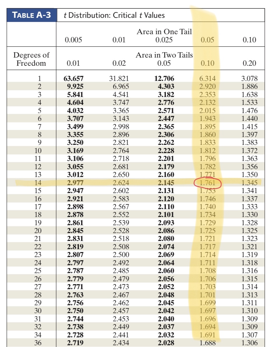
- [latex]t_{\frac{\alpha}{2}} = 1.761[/latex] based on the intersection of the df and [latex]\alpha[/latex] above
- [latex]E = t_{\frac{\alpha}{2}} \times\frac{s}{\sqrt{n}} = 1.761 \times \frac{1.67}{\sqrt{15}} = 0.7593[/latex]
Here’s the confidence interval, in the three different forms:
| Basic Form | Inequalities | Interval Notation |
| [latex]8.23 \pm 0.7593[/latex] | [latex]8.23 - 0.7593 \le \mu \le 8.23 + 0.7593[/latex] | [latex](8.23 - 0.7593, 8.23 + 0.7593)[/latex] |
| [latex]7.471 \le \mu \le 8.989[/latex] | [latex](7.471, 8.989)[/latex] |
Notice that in this example we did NOT convert into a percent. This problem deals with means (averages) which are not percents. So after we do the computation, we leave the numbers in decimal form. We just need to make sure we round according to instructions or by our default.
So what does this mean, what did we find out? We are 90% confident that the true mean sensory rate for the population is between 7.471 and 8.989.
Example 2: Screen time during lockdown
A recent online survey conducted in India asked randomly selected respondents to self-report their screen time and how it changed during a lockdown due to COVID. The survey involved [latex]n = 1000[/latex] respondents aged 13-25 years. The average screen time for respondents was [latex]\bar{x} = 5.13[/latex] hours, which is considered very high when compared to their pre-lockdown average of [latex]3.5[/latex] hours. The standard deviation for their screen time was found to be [latex]s = 1.9[/latex] hours. Use the sample data to construct a 95% confidence interval for the true average screen time for the population.
Solution
In this example, we are told that a random sample is part of the data. We are also told that the sample size is [latex]n = 1000[/latex], so the requirements are met. Here we are given all the information we need. Let’s go through and identify the values we need to work this out.
- [latex]n = 1000[/latex]
- [latex]\bar{x} = 5.13[/latex]
- [latex]s = 1.9[/latex]
- [latex]df = n - 1 = 1000 -1 = 999[/latex]
- [latex]\alpha = 1 - 0.95 = 0.05[/latex]
- 0.95 is the 95% confidence level written as a decimal
- We subtract from 1 to find [latex]\alpha[/latex]
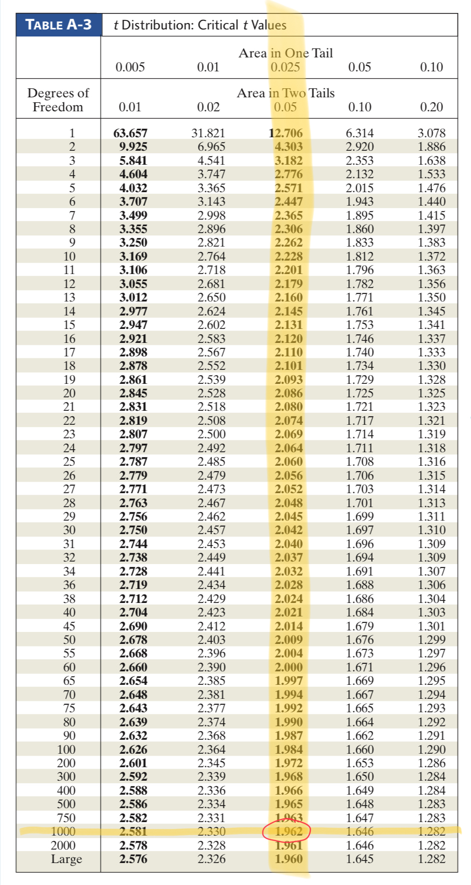
- [latex]t_{\frac{\alpha}{2}} = 1.962[/latex] based on the intersection of the df and [latex]\alpha[/latex] above
- Since [latex]df = 999[/latex] was not actually on the chart, we use the closest value, which is 1000
- [latex]E = t_{\frac{\alpha}{2}} \times\frac{s}{\sqrt{n}} = 1.962 \times \frac{1.9}{\sqrt{1000}} = 0.1179[/latex]
Here’s the confidence interval, in the three different forms:
| Basic Form | Inequalities | Interval Notation |
| [latex]5.13 \pm 0.1179[/latex] | [latex]5.13 - 0.1179 \le \mu \le 5.13 + 0.1179[/latex] | [latex](5.13 - 0.1179, 5.13 + 0.1179)[/latex] |
| [latex]5.012 \le \mu \le 5.248[/latex] | [latex](5.012, 5.248)[/latex] |
Notice that in this example we did NOT convert into a percent. This problem deals with means (averages) which are not percents. So after we do the computation, we leave the numbers in decimal form. We just need to make sure we round according to instructions or by our default.
So what does this mean, what did we find out? We are 95% confident that the true average screen time for the population is between 5.012 hours and 5.248 hours.
Example 3: social media use
A 2020 survey found that [latex]n = 67[/latex] respondents spent an average of [latex]\bar{x} = 2.5[/latex] hours each day on social media, with a standard deviation of [latex]s = 0.35[/latex] hours. Use the sample data to construct a 99% confidence interval for the true average daily time on social media for the population.
Solution
In this example, we are not told that a random sample is part of the data. However, we are told that the sample size is [latex]n = 67[/latex], so the requirements are met. Here we are given all the information we need. Let’s go through and identify the values we need to work this out.
- [latex]n = 67[/latex]
- [latex]\bar{x} = 2.5[/latex]
- [latex]s = 0.35[/latex]
- [latex]df = n - 1 = 67 -1 = 66[/latex]
- [latex]\alpha = 1 - 0.99 = 0.01[/latex]
- 0.99 is the 99% confidence level written as a decimal
- We subtract from 1 to find [latex]\alpha[/latex]
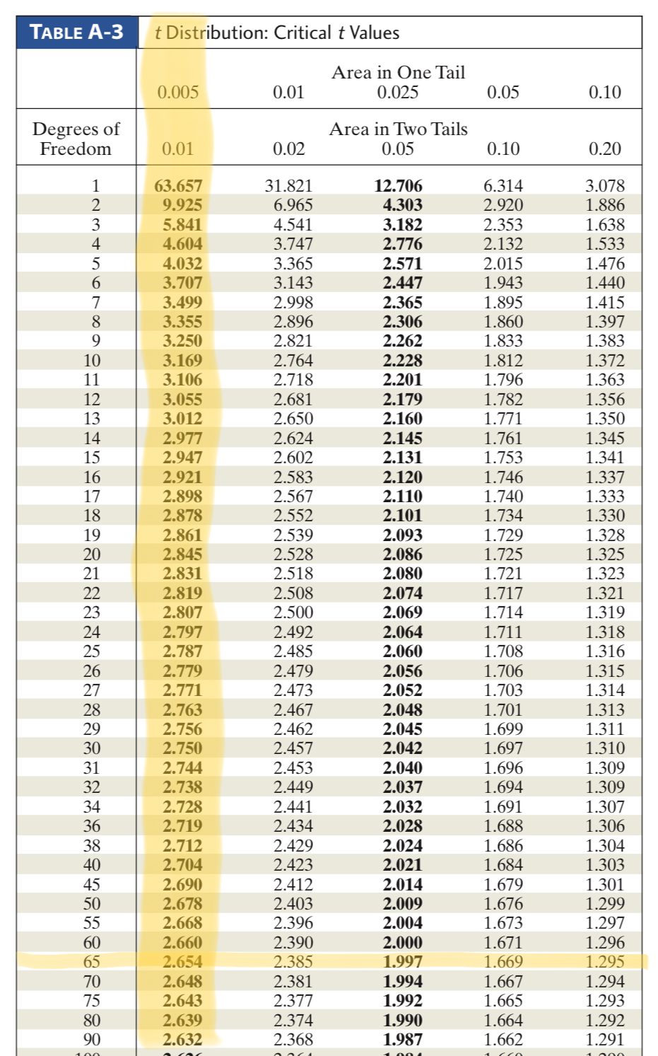
- [latex]t_{\frac{\alpha}{2}} = 2.654[/latex] based on the intersection of the df and [latex]\alpha[/latex] above
- Since [latex]df = 66[/latex] was not actually on the chart, we use the closest value, which is 65
- [latex]E = t_{\frac{\alpha}{2}} \times\frac{s}{\sqrt{n}} = 2.654 \times \frac{0.35}{\sqrt{67}} = 0.1135[/latex]
Here’s the confidence interval, in the three different forms:
| Basic Form | Inequalities | Interval Notation |
| [latex]2.5 \pm 0.1135[/latex] | [latex]2.5 - 0.1135 \le \mu \le 2.5 + 0.1135[/latex] | [latex](2.5 - 0.1135, 2.5 + 0.1135)[/latex] |
| [latex]2.387 \le \mu \le 2.614[/latex] | [latex](2.387, 2.614)[/latex] |
Notice that in this example we did NOT convert into a percent. This problem deals with means (averages) which are not percents. So after we do the computation, we leave the numbers in decimal form. We just need to make sure we round according to instructions or by our default.
So what does this mean, what did we find out? We are 99% confident that the true average daily time on social media for the population is between 2.387 hours and 2.614 hours.
- Adapted from OpenStax Statistics by Barbara Illowsky & Susan Dean, licensed under CC BY 4.0 ↵
