Inference for Comparing 2 Population Means (HT for 2 Means, independent samples)
More of the good stuff! We will need to know how to label the null and alternative hypothesis, calculate the test statistic, and then reach our conclusion using the critical value method or the p-value method.
The Test Statistic for a Test of 2 Means from Independent Samples:
[latex]t = \displaystyle \frac{(\bar{x_1} - \bar{x_2}) - (\mu_1 - \mu_2)}{\sqrt{\displaystyle \frac{s_1^2}{n_1} + \displaystyle \frac{s_2^2}{n_2}}}[/latex]
What the different symbols mean:
[latex]n_1[/latex] is the sample size for the first group
[latex]n_2[/latex] is the sample size for the second group
[latex]df[/latex], the degrees of freedom, is the smaller of [latex]n_1 - 1[/latex] and [latex]n_2 - 1[/latex]
[latex]\mu_1[/latex] is the population mean from the first group
[latex]\mu_2[/latex] is the population mean from the second group
[latex]\bar{x_1}[/latex] is the sample mean for the first group
[latex]\bar{x_2}[/latex] is the sample mean for the second group
[latex]s_1[/latex] is the sample standard deviation for the first group
[latex]s_2[/latex] is the sample standard deviation for the second group
[latex]\alpha[/latex] is the significance level, usually given within the problem, or if not given, we assume it to be 5% or 0.05
Assumptions when conducting a Test for 2 Means from Independent Samples:
- We do not know the population standard deviations, and we do not assume they are equal
- The two samples or groups are independent
- Both samples are simple random samples
- Both populations are Normally distributed OR both samples are large ([latex]n_1 > 30[/latex] and [latex]n_2 > 30[/latex])
Steps to conduct the Test for 2 Means from Independent Samples:
- Identify all the symbols listed above (all the stuff that will go into the formulas). This includes [latex]n_1[/latex] and [latex]n_2[/latex], [latex]df[/latex], [latex]\mu_1[/latex] and [latex]\mu_2[/latex], [latex]\bar{x_1}[/latex] and [latex]\bar{x_2}[/latex], [latex]s_1[/latex] and [latex]s_2[/latex], and [latex]\alpha[/latex]
- Identify the null and alternative hypotheses
- Calculate the test statistic, [latex]t = \displaystyle \frac{(\bar{x_1} - \bar{x_2}) - (\mu_1 - \mu_2)}{\sqrt{\displaystyle \frac{s_1^2}{n_1} + \displaystyle \frac{s_2^2}{n_2}}}[/latex]
- Find the critical value(s) OR the p-value OR both
- Apply the Decision Rule
- Write up a conclusion for the test
Example 1: Study on the effectiveness of stents for stroke patients[1]
In this study, researchers randomly assigned stroke patients to two groups: one received the current standard care (control) and the other received a stent surgery in
addition to the standard care (stent treatment). If the stents work, the treatment group should have a lower average disability score. Do the results give convincing statistical evidence that the stent treatment reduces the average disability from stroke?
| Stent (group 1) | Control (group 2) | |
| Mean Disability Score | 2.26 | 3.23 |
| Standard Deviation Disability Score | 1.78 | 1.78 |
| Sample Size, n | 98 | 93 |
Solution
Since we are being asked for convincing statistical evidence, a hypothesis test should be conducted. In this case, we are dealing with averages from two samples or groups (the patients with stent treatment and patients receiving the standard care), so we will conduct a Test of 2 Means.
- [latex]n_1 = 98[/latex] is the sample size for the first group
- [latex]n_2 = 93[/latex] is the sample size for the second group
- [latex]df[/latex], the degrees of freedom, is the smaller of [latex]98 - 1 = 97[/latex] and [latex]93 - 1 = 92[/latex], so [latex]df = 92[/latex]
- [latex]\bar{x_1} = 2.26[/latex] is the sample mean for the first group
- [latex]\bar{x_2} = 3.23[/latex] is the sample mean for the second group
- [latex]s_1 = 1.78[/latex] is the sample standard deviation for the first group
- [latex]s_2 = 1.78[/latex] is the sample standard deviation for the second group
- [latex]\alpha = 0.05[/latex] (we were not told a specific value in the problem, so we are assuming it is 5%)
- One additional assumption we extend from the null hypothesis is that [latex]\mu_1 - \mu_2 = 0[/latex]; this means that in our formula, those variables cancel out
- Null and Alternative Hypothesis: In a 2-sample problem, the null hypothesis will always be the assumption that the groups are the same, or that they have the same averages. In this case we are being asked if there is evidence that the stent treatment group has a lower average disability score than the standard treatment group, so the alternative hypothesis uses a [latex]<[/latex] symbol.
- [latex]H_{0}: \mu_1 = \mu_2[/latex]
- [latex]H_{A}: \mu_1 < \mu_2[/latex]
- Test Statistic
- [latex]t = \displaystyle \frac{(\bar{x_1} - \bar{x_2}) - (\mu_1 - \mu_2)}{\sqrt{\displaystyle \frac{s_1^2}{n_1} + \displaystyle \frac{s_2^2}{n_2}}} = \displaystyle \frac{(2.26 - 3.23) - 0)}{\sqrt{\displaystyle \frac{1.78^2}{98} + \displaystyle \frac{1.78^2}{93}}} = -3.76[/latex]
- P-Value: Here we will get a little bit of practice using some of the power of Excel, Google Sheets, or StatDisk to give us the P-Value.
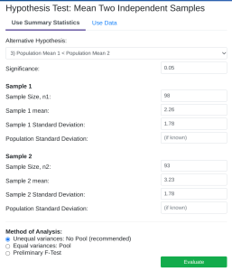
- StatDisk: We can conduct this test using StatDisk. The nice thing about StatDisk is that it will also compute the test statistic. From the main menu above we click on Analysis, Hypothesis Testing, and then Mean Two Independent Samples. From there enter the 0.05 significance, along with the specific values as outlined in the picture below in Step 2. Notice the alternative hypothesis is the [latex]<[/latex] option. Enter the sample size, mean, and standard deviation for each group, and make sure that unequal variances is selected. Now we click on Evaluate. If you check the values, the test statistic is reported in the Step 3 display, as well as the P-Value of 0.00011.
-
Step 1 Step 2 Step 3 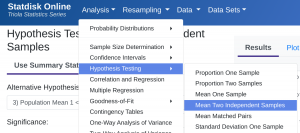
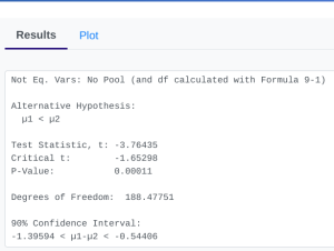
- Applying the Decision Rule: We now compare this to our significance level, which is 0.05. If the p-value is smaller or equal to the alpha level, we have enough evidence for our claim, otherwise we do not. Here, [latex]p-value = 0.00011[/latex], which is definitely smaller than [latex]\alpha = 0.05[/latex], so we have enough evidence for the alternative hypothesis…but what does this mean?
- Conclusion: Because our p-value of [latex]0.00011[/latex] is less than our [latex]\alpha[/latex] level of [latex]0.05[/latex], we reject [latex]H_{0}[/latex]. We have convincing statistical evidence that the stent treatment reduces the average disability from stroke.
Example 2: Home Run Distances
In 1998, Sammy Sosa and Mark McGwire (2 players in Major League Baseball) were on pace to set a new home run record. At the end of the season McGwire ended up with 70 home runs, and Sosa ended up with 66. The home run distances were recorded and compared (sometimes a player’s home run distance is used to measure their “power”). Do the results give convincing statistical evidence that the home run distances are different from each other? Who would you say “hit the ball farther” in this comparison?
| McGwire (group 1) | Sosa (group 2) | |
| Mean Home Run Distance | 418.5 | 404.8 |
| Standard Deviation Home Run Distance | 45.5 | 35.7 |
| Sample Size, n | 70 | 66 |
Solution
Since we are being asked for convincing statistical evidence, a hypothesis test should be conducted. In this case, we are dealing with averages from two samples or groups (the home run distances), so we will conduct a Test of 2 Means.
- [latex]n_1 = 70[/latex] is the sample size for the first group
- [latex]n_2 = 66[/latex] is the sample size for the second group
- [latex]df[/latex], the degrees of freedom, is the smaller of [latex]70 - 1 = 69[/latex] and [latex]66 - 1 = 65[/latex], so [latex]df = 65[/latex]
- [latex]\bar{x_1} = 418.5[/latex] is the sample mean for the first group
- [latex]\bar{x_2} = 404.8[/latex] is the sample mean for the second group
- [latex]s_1 = 45.5[/latex] is the sample standard deviation for the first group
- [latex]s_2 = 35.7[/latex] is the sample standard deviation for the second group
- [latex]\alpha = 0.05[/latex] (we were not told a specific value in the problem, so we are assuming it is 5%)
- One additional assumption we extend from the null hypothesis is that [latex]\mu_1 - \mu_2 = 0[/latex]; this means that in our formula, those variables cancel out
- Null and Alternative Hypothesis: In a 2-sample problem, the null hypothesis will always be the assumption that the groups are the same, or that they have the same averages. In this case we are being asked if there is evidence that the distances are different, so the alternative hypothesis uses a [latex]\neq[/latex] symbol.
- [latex]H_{0}: \mu_1 = \mu_2[/latex]
- [latex]H_{A}: \mu_1 \neq \mu_2[/latex]
- Test Statistic
- [latex]t = \displaystyle \frac{(\bar{x_1} - \bar{x_2}) - (\mu_1 - \mu_2)}{\sqrt{\displaystyle \frac{s_1^2}{n_1} + \displaystyle \frac{s_2^2}{n_2}}} = \displaystyle \frac{(418.5 - 404.8) - 0)}{\sqrt{\displaystyle \frac{45.5^2}{70} + \displaystyle \frac{35.7^2}{65}}} = 1.95[/latex]
- P-Value: Here we will get a little bit of practice using some of the power of Excel, Google Sheets, or StatDisk to give us the P-Value.
- StatDisk: We can conduct this test using StatDisk. The nice thing about StatDisk is that it will also compute the test statistic. From the main menu above we click on Analysis, Hypothesis Testing, and then Mean Two Independent Samples. From there enter the 0.05 significance, along with the specific values as outlined in the picture below in Step 2. Notice the alternative hypothesis is the [latex]\neq[/latex] option. Enter the sample size, mean, and standard deviation for each group, and make sure that unequal variances is selected. Now we click on Evaluate. If you check the values, the test statistic is reported in the Step 3 display, as well as the P-Value of 0.05221.
-
Step 1 Step 2 Step 3 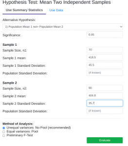
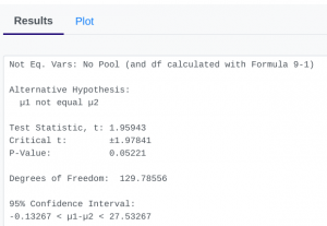
- Applying the Decision Rule: We now compare this to our significance level, which is 0.05. If the p-value is smaller or equal to the alpha level, we have enough evidence for our claim, otherwise we do not. Here, [latex]p-value = 0.05221[/latex], which is larger than [latex]\alpha = 0.05[/latex], so we do not have enough evidence for the alternative hypothesis…but what does this mean?
- Conclusion: Because our p-value of [latex]0.05221[/latex] is larger than our [latex]\alpha[/latex] level of [latex]0.05[/latex], we fail to reject [latex]H_{0}[/latex]. We do not have convincing statistical evidence that the home run distances are different.
- Follow-up commentary: But what does this mean? There actually was a difference, right? If we take McGwire’s average and subtract Sosa’s average we get a difference of 13.7. What this result indicates is that the difference is not statistically significant; it could be due more to random chance than something meaningful. Other factors, such as sample size, could also be a determining factor (with a larger sample size, the difference may have been more meaningful).
- Adapted from the Skew The Script curriculum (skewthescript.org), licensed under CC BY-NC-Sa 4.0 ↵
