Inference for Comparing Matched Pairs (HT for 2 Means, dependent samples)
More of the good stuff! We will need to know how to label the null and alternative hypothesis, calculate the test statistic, and then reach our conclusion using the critical value method or the p-value method.
The Test Statistic for a Test of Matched Pairs (2 Means from Dependent Samples):
[latex]t = \displaystyle \frac{\bar{x} - 0}{\frac{s}{\sqrt{n}}}[/latex]
What the different symbols mean:
[latex]n[/latex] is the sample size, or the number of pairs of data
[latex]df = n - 1[/latex] is the degrees of freedom
[latex]\mu_d[/latex] is the mean value of the differences for the population of all matched pairs of data
[latex]\bar{x}[/latex] is the sample mean of the computed differences for the paired sample data
[latex]s[/latex] is the sample standard deviation of the computed differences for the paired sample data
[latex]\alpha[/latex] is the significance level, usually given within the problem, or if not given, we assume it to be 5% or 0.05
Assumptions when conducting a Test for Matched Pairs:
- The two samples or groups are dependent
- The matched pairs are a simple random sample
- The number of pairs of sample data is large ([latex]n > 30[/latex]), OR the pairs of values have differences from a population that is approximately normal.
Steps to conduct the Test for Matched Pairs:
- Identify all the symbols listed above (all the stuff that will go into the formulas). This includes [latex]n[/latex], [latex]df[/latex], [latex]\mu_d[/latex], [latex]\bar{x}[/latex], [latex]s[/latex], and [latex]\alpha[/latex]
- Identify the null and alternative hypotheses
- Calculate the test statistic, [latex]t = \displaystyle \frac{\bar{x} - 0}{\frac{s}{\sqrt{n}}}[/latex]
- Find the critical value(s) OR the p-value OR both
- Apply the Decision Rule
- Write up a conclusion for the test
Example 1: Global Warming and Climate Change[1]
In Michael Crichton’s book “The State of Fear,” a reference is made to reported temperatures declining in Punta Arenas, at a weather station in South America. The reference in the book indicates that the temperature decreases there discredit climate change. There is a danger, however, in using data from only one source and one time period when making statements that might have worldwide impact. Instead of using data from one location and one time, it might be better to look at trends from many stations and from multiple time periods. The table below shows collected temperature readings from 32 NASA-GISS stations based on a random sample of latitude-longitude coordinates. The table is a matched-pairs design, and the differences can be analyzed to determine if we have statistically convincing evidence of true global warming (on average). [NOTE: since we are talking about global warming, the implication is that temperatures would be rising, so the mean difference would be thought of as an increase for the alternative hypothesis.] You can get a copy of the table in Google Sheets format here.
| Temperature Readings from NASA-GISS Stations | |||
| Selected Station | 1901 – 1950 Temperature | 1951 – 2000 Temperature | Difference (°C) |
| Sable Island | 6.803 | 7.420 | 0.617 |
| Manila Intl Airport | 26.779 | 27.416 | 0.637 |
| Hobart Ellerslie | 12.549 | 13.062 | 0.538 |
| Bulawayo Goetz | 18.891 | 19.183 | 0.292 |
| Veraval | 26.404 | 26.779 | 0.375 |
| Yokohama | 14.534 | 15.428 | 0.894 |
| Punta Arenas | 6.828 | 6.752 | -0.077 |
| Aldergrove | 8.888 | 9.012 | 0.124 |
| Harare Kutsaga | 18.816 | 19.055 | 0.239 |
| Bahia Blanca Aero | 14.963 | 15.204 | 0.241 |
| Maliye Karmakuly | -5.036 | -5.044 | -0.008 |
| Hobarttasmanwas | 12.439 | 12.638 | 0.199 |
| Svaytoy | -0.263 | 0.263 | 0.527 |
| Apia | 26.380 | 26.479 | 0.099 |
| Aparri | 25.288 | 26.091 | 0.803 |
| Syktyvkar | 0.435 | 0.894 | 0.460 |
| Upernavik | -7.012 | -7.286 | -0.274 |
| Gabo Island | 14.925 | 14.924 | -0.001 |
| Antananariovoville | 17.387 | 17.741 | 0.354 |
| Kumasi | 25.652 | 25.854 | 0.202 |
| Khartoum | 28.535 | 28.874 | 0.339 |
| Mahe Seychellesbri | 26.414 | 26.872 | 0.459 |
| Onslow | 24.154 | 24.540 | 0.387 |
| Rarotonga Intl | 24.105 | 24.157 | 0.052 |
| Ponta Delgada | 14.942 | 15.676 | 0.734 |
| Viljujsk | -8.854 | -9.057 | -0.203 |
| Andenes | 2.600 | 3.160 | 0.560 |
| Kyzylorda | 9.631 | 10.411 | 0.780 |
| Port Blair | 26.506 | 26.778 | 0.271 |
| Chatham Islands | 10.392 | 11.132 | 0.739 |
| Perm | 1.670 | 2.208 | 0.538 |
| Cape Leeuwin | 16.608 | 16.983 | 0.375 |
Solution
Since we are being asked for convincing statistical evidence, a hypothesis test should be conducted. In this case, we are dealing with gains (differences) from pairs of data, the pre- and post-tests, so we will conduct a Test for Matched Pairs.
- [latex]n = 32[/latex] is the sample size, or the number of pairs of data
- [latex]df = n - 1 = 32 - 1 = 31[/latex] is the degrees of freedom
- [latex]\bar{x} = 0.35[/latex] is the sample mean of the computed differences for the paired sample data
- You can either manually add up and divide by how many, or you can use the Excel or Sheets formula =average() and make sure the appropriate numbers are entered or selected
- You can also do the same for standard deviation; use the =stdev() formula in Excel or Sheets
- [latex]s = 0.296[/latex] is the sample standard deviation of the computed differences for the paired sample data
- [latex]\alpha[/latex] is the significance level, usually given within the problem, or if not given, we assume it to be 5% or 0.05
- Null and Alternative Hypothesis: In a Matched Pairs problem, the null hypothesis will always be the assumption that there is no increase, decrease, or difference, or that the mean difference is zero. In this case we are being asked if there is evidence for global warming (or an increase in temperatures), so the alternative hypothesis uses a [latex]>[/latex] symbol.
- [latex]H_{0}: \mu_d = 0[/latex]
- [latex]H_{A}: \mu_d > 0[/latex]
- Test Statistic
- [latex]t = \displaystyle \frac{\bar{x} - 0}{\frac{s}{\sqrt{n}}} = \displaystyle \frac{0.35 - 0}{\frac{0.296}{\sqrt{32}}} = 6.689[/latex]
- P-Value: Here we will get a little bit of practice using some of the power of Excel, Google Sheets, or StatDisk to give us the P-Value.
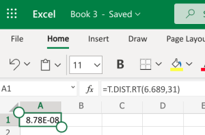
- Microsoft Excel: You don’t need to have the Data Analysis ToolPack installed for this. Since we already have the differences calculated and we have the mean and standard deviation on those differences (the gain column), we can use the regular t-distribution on those values, including the test statistic and the degrees of freedom. We can use the built-in T.DIST.RT function to help calculate it. The “RT” in the formula is for the “more than” problems. The function will be typed into an empty cell in Excel (either installed on your computer, or using the online version) as =T.DIST.RT(x,deg_freedom), where x is the [latex]t[/latex] test statistic we just calculated (but always entered as a positive value), and deg_freedom is the [latex]df[/latex] we calculated earlier. The “RT” in the formula is for the “more than” problems. Step 1 illustrates how we would enter =T.DIST.RT(6.689,31). Step 2 gives us 8.78E-08, which is scientific notation. This means we move the decimal to the left 8 spaces, and we have a bunch of zeros in front of the 878. This means our actual value, if we round to 4 places, would be 0.0000, which is the [latex]p-value[/latex].
-
Step 1 Step 2 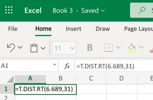
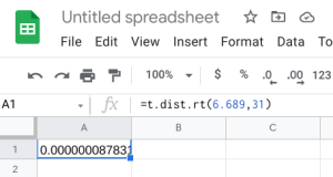
- Google Sheets: You can also do this using the exact same built-in function within Google Sheets. We can use the built-in T.DIST.RT function to help calculate it. The function will be typed into an empty cell in Google Sheets as =T.DIST.RT(x,deg_freedom), where x is the [latex]t[/latex] test statistic we just calculated (but always entered as a positive value), and deg_freedom is the [latex]df[/latex] we calculated earlier. The “RT” in the formula is for the “more than” problems. Step 1 illustrates how we would enter =T.DIST.RT(6.689,31). Step 2 gives us 0.0000, which is the [latex]p-value[/latex].
-
Step 1 Step 2 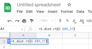
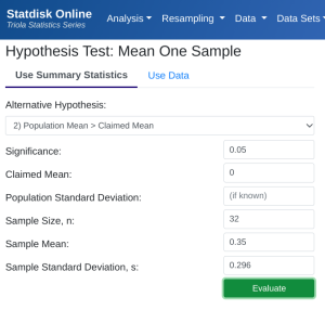
- StatDisk: We can conduct this test using StatDisk, but slightly modified from the full process. Since we already have the mean and standard deviation on the differences (the gain), we can use the regular test for one mean. The nice thing about StatDisk is that it will also compute the test statistic. From the main menu above we click on Analysis, Hypothesis Testing, and then Mean One Sample (the calculated “gain” is like a single sample now). From there enter the 0.05 significance, along with the specific values as outlined in the picture below in Step 2. Notice the alternative hypothesis is the [latex]>[/latex] option. Enter the sample size, mean, and standard deviation. Now we click on Evaluate. If you check the values, the test statistic is reported in the Step 3 display, as well as the P-Value of 0.0000.
-
Step 1 Step 2 Step 3 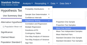
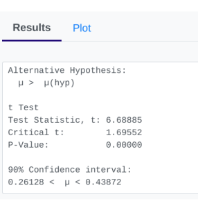
- Applying the Decision Rule: We now compare this to our significance level, which is 0.05. If the p-value is smaller or equal to the alpha level, we have enough evidence for our claim, otherwise we do not. Here, [latex]p-value = 0.0000[/latex], which is smaller than [latex]\alpha = 0.05[/latex], so we have enough evidence for the alternative hypothesis…but what does this mean?
- Conclusion: Because our p-value of [latex]0.0000[/latex] is smaller than our [latex]\alpha[/latex] level of [latex]0.05[/latex], we reject [latex]H_{0}[/latex]. We have convincing statistical evidence of true global warming (on average).
.
Example 2: Summer Institute for Foreign Language Instruction[2]
At UA High School there is a summer institute to improve the skills of high school teachers of foreign languages. One summer institute hosted 20 French teachers for 4 weeks. At the beginning of the period, teachers were given a baseline exam covering Modern Language listening. After 4 weeks of immersion in French in and out of class, the exam was administered once again. The table below gives pretest and posttest scores. Do the results give convincing statistical evidence that the institute improved the teacher’s comprehension of spoken French? You can get a copy of the data table in Google Sheets format here.
| Modern Language Association listening scores for French teachers | |||
| Teacher | Pretest | Posttest | Gain |
| 1 | 32 | 34 | 2 |
| 2 | 31 | 31 | 0 |
| 3 | 29 | 35 | 6 |
| 4 | 10 | 16 | 6 |
| 5 | 30 | 33 | 3 |
| 6 | 30 | 36 | 6 |
| 7 | 20 | 26 | 6 |
| 8 | 24 | 27 | 3 |
| 9 | 24 | 24 | 0 |
| 10 | 31 | 32 | 1 |
| 11 | 33 | 36 | 3 |
| 12 | 30 | 31 | 1 |
| 13 | 22 | 24 | 2 |
| 14 | 15 | 15 | 0 |
| 15 | 25 | 28 | 3 |
| 16 | 32 | 34 | 2 |
| 17 | 32 | 26 | -6 |
| 18 | 23 | 26 | 3 |
| 19 | 20 | 26 | 6 |
| 20 | 23 | 26 | 3 |
Solution
Since we are being asked for convincing statistical evidence, a hypothesis test should be conducted. In this case, we are dealing with gains (differences) from pairs of data, the pre- and post-tests, so we will conduct a Test for Matched Pairs.
- [latex]n = 20[/latex] is the sample size, or the number of pairs of data
- [latex]df = n - 1 = 20 - 1 = 19[/latex] is the degrees of freedom
- [latex]\bar{x} = 2.5[/latex] is the sample mean of the computed differences for the paired sample data
- You can either manually add up and divide by how many, or you can use the Excel or Sheets formula =average() and make sure the appropriate numbers are entered or selected
- You can also do the same for standard deviation; use the =stdev() formula in Excel or Sheets
- [latex]s = 2.893[/latex] is the sample standard deviation of the computed differences for the paired sample data
- [latex]\alpha[/latex] is the significance level, usually given within the problem, or if not given, we assume it to be 5% or 0.05
- Null and Alternative Hypothesis: In a Matched Pairs problem, the null hypothesis will always be the assumption that there is no increase, decrease, or difference, or that the mean difference is zero. In this case we are being asked if there is evidence that there is an improvement (or an increase) in scores, so the alternative hypothesis uses a [latex]>[/latex] symbol.
- [latex]H_{0}: \mu_d = 0[/latex]
- [latex]H_{A}: \mu_d > 0[/latex]
- Test Statistic
- [latex]t = \displaystyle \frac{\bar{x} - 0}{\frac{s}{\sqrt{n}}} = \displaystyle \frac{2.5 - 0}{\frac{2.893}{\sqrt{20}}} = 3.86[/latex]
- P-Value: Here we will get a little bit of practice using some of the power of Excel, Google Sheets, or StatDisk to give us the P-Value.
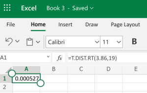
- Microsoft Excel: You don’t need to have the Data Analysis ToolPack installed for this. Since we already have the differences calculated and we have the mean and standard deviation on those differences (the gain column), we can use the regular t-distribution on those values, including the test statistic and the degrees of freedom. We can use the built-in T.DIST.RT function to help calculate it. The “RT” in the formula is for the “more than” problems. The function will be typed into an empty cell in Excel (either installed on your computer, or using the online version) as =T.DIST.RT(x,deg_freedom), where x is the [latex]t[/latex] test statistic we just calculated (but always entered as a positive value), and deg_freedom is the [latex]df[/latex] we calculated earlier. The “RT” in the formula is for the “more than” problems. Step 1 illustrates how we would enter =T.DIST.RT(3.86,19). Step 2 gives us 0.000527, which is the [latex]p-value[/latex].
-
Step 1 Step 2 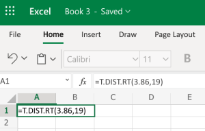
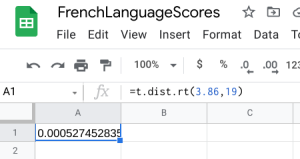
- Google Sheets: You can also do this using the exact same built-in function within Google Sheets. We can use the built-in T.DIST.RT function to help calculate it. The function will be typed into an empty cell in Google Sheets as =T.DIST.RT(x,deg_freedom), where x is the [latex]t[/latex] test statistic we just calculated (but always entered as a positive value), and deg_freedom is the [latex]df[/latex] we calculated earlier. The “RT” in the formula is for the “more than” problems. Step 1 illustrates how we would enter =T.DIST.RT(3.86,19). Step 2 gives us 0.000527, which is the [latex]p-value[/latex].
-
Step 1 Step 2 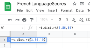
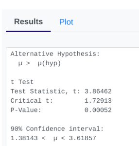
- StatDisk: We can conduct this test using StatDisk, but slightly modified from the full process. Since we already have the mean and standard deviation on the differences (the gain), we can use the regular test for one mean. The nice thing about StatDisk is that it will also compute the test statistic. From the main menu above we click on Analysis, Hypothesis Testing, and then Mean One Sample (the calculated “gain” is like a single sample now). From there enter the 0.05 significance, along with the specific values as outlined in the picture below in Step 2. Notice the alternative hypothesis is the [latex]>[/latex] option. Enter the sample size, mean, and standard deviation. Now we click on Evaluate. If you check the values, the test statistic is reported in the Step 3 display, as well as the P-Value of 0.00052.
-
Step 1 Step 2 Step 3 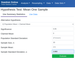
- Applying the Decision Rule: We now compare this to our significance level, which is 0.05. If the p-value is smaller or equal to the alpha level, we have enough evidence for our claim, otherwise we do not. Here, [latex]p-value = 0.000527[/latex], which is smaller than [latex]\alpha = 0.05[/latex], so we have enough evidence for the alternative hypothesis…but what does this mean?
- Conclusion: Because our p-value of [latex]0.000527[/latex] is smaller than our [latex]\alpha[/latex] level of [latex]0.05[/latex], we reject [latex]H_{0}[/latex]. We have convincing statistical evidence that the institute improved the teacher’s comprehension of spoken French.
- Adapted from the Skew The Script curriculum (skewthescript.org), licensed under CC BY-NC-Sa 4.0 ↵
- Adapted from The Introduction to the Practice of Statistics, 3rd Edition, by Moore & McCabe ↵
