Inference for a Population Mean (HT for 1 Mean, Sigma Unknown)
Now we get to the good stuff! We will need to know how to label the null and alternative hypothesis, calculate the test statistic, and then reach our conclusion using the critical value method or the p-value method.
The Test Statistic for Testing 1 Mean, σ Unknown:
[latex]t = \displaystyle \frac{\bar{x} - \mu}{\frac{s}{\sqrt{n}}}[/latex]
What the different symbols mean:
[latex]n[/latex] is the sample size (number of people, items, etc… in the study)
[latex]df = n - 1[/latex] is the degrees of freedom
[latex]\mu[/latex] is the population mean
[latex]\bar{x}[/latex] is the sample mean (also known as average)
[latex]s[/latex] is the sample standard deviation
[latex]\alpha[/latex] is the significance level, usually given within the problem, or if not given, we assume it to be 5% or 0.05
Assumptions when conducting a Test for 1 Mean, σ Unknown:
- We have a simple random sample
- We have a normal distribution OR [latex]n\ge 30[/latex]
Steps to conduct a Test for 1 Mean, σ Unknown:
- Identify all the symbols listed above (all the stuff that will go into the formulas). This includes [latex]n[/latex], [latex]df[/latex], [latex]\mu[/latex], [latex]\bar{x}[/latex], [latex]s[/latex], and [latex]\alpha[/latex]
- Identify the null and alternative hypotheses
- Calculate the test statistic, [latex]t = \displaystyle \frac{\bar{x} - \mu}{\frac{s}{\sqrt{n}}}[/latex]
- Find the critical value(s) OR the p-value OR both
- Apply the Decision Rule
- Write up a conclusion for the test
Example 1: The Cost of a Big Mac in Imperial County vs the World
One of the things that chain restaurants and fast food bring us is some consistency. In many cases, we would also expect the prices of items to be consistent at different locations. This may not always be the case. A Big Mac in Imperial County will likely cost about $5.99. How does this compare to other locations, even other countries? Is it higher or lower? Data collected from [latex]n = 112[/latex] countries during 2020 revealed a mean cost of [latex]\bar{x} = \$3.58[/latex] and a standard deviation of [latex]s = \$1.07[/latex]. Is there convincing statistical evidence that the cost of a Big Mac differs in places other than Imperial County?
Solution
Since we are being asked for convincing statistical evidence, a hypothesis test should be conducted. In this case, we are dealing with averages or means from one sample or group (McDonald’s around the world), so we will conduct a Test for 1 Mean, [latex]\sigma[/latex] Unknown.
- [latex]n = 112[/latex]
- [latex]df = n -1 = 112 - 1 = 111[/latex]
- [latex]\bar{x} = \$3.58[/latex]
- [latex]s = \$1.07[/latex]
- [latex]\alpha = 0.05[/latex] (we were not told a specific value in the problem, so we are assuming it is 5%)
- Null and Alternative Hypothesis: Since the Big Mac in Imperial County costs $5.99, and the question is whether the Big Mac has a different cost in other countries, the claim that goes along with the alternative hypothesis is that [latex]\mu[/latex] is not equal to $5.99. In our example here, the idea that “nothing is different” would be equivalent to saying that [latex]\mu[/latex] is the same as (equal to) $5.99.
- [latex]H_{0}: \mu = \$5.99[/latex]
- [latex]H_{A}: \mu \neq \$5.99[/latex]
- [latex]\mu = \$5.99[/latex] (from the null hypothesis)
- Test Statistic
- [latex]t = \displaystyle \frac{\bar{x} - \mu}{\frac{s}{\sqrt{n}}}\ = \displaystyle \frac{3.58 - 5.99}{\frac{1.07}{\sqrt{112}}} = -23.836[/latex] (generally we round [latex]t[/latex] to 3 places)
- P-Value: Here we will get a little bit of practice using some of the power of Excel, Google Sheets, or StatDisk to give us the P-Value.
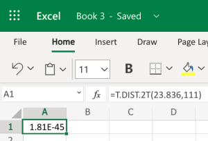
- Microsoft Excel: You don’t need to have the Data Analysis ToolPack installed for this. We can use the built-in T.DIST.2T function to help calculate it. The function will be typed into an empty cell in Excel (either installed on your computer, or using the online version) as =T.DIST.2T(x,deg_freedom), where x is the [latex]t[/latex] test statistic we just calculated (but always entered as a positive value), and deg_freedom is the [latex]df[/latex] we calculated earlier. We would enter =T.DIST.2T(23.836,111). Notice the 1.81E-45 in the second picture. This is scientific notation; the -45 indicates we move the decimal 45 spaces to the left, which basically leaves a bunch of zeros. This gives us a [latex]p-value[/latex] of [latex]0.000[/latex].
-
Step 1 Step 2 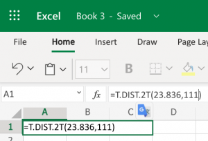
-
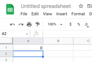
- Google Sheets: You can also do this using the exact same built-in function within Google Sheets. We can use the built-in T.DIST.2T function to help calculate it. The function will be typed into an empty cell in Google Sheets as =T.DIST.2T(x,deg_freedom), where x is the [latex]t[/latex] test statistic we just calculated (but always entered as a positive value), and deg_freedom is the [latex]df[/latex] we calculated earlier. We would enter =T.DIST.2T(23.836,111). This gives us a [latex]p-value[/latex] of [latex]0.000[/latex].
-
Step 1 Step 2 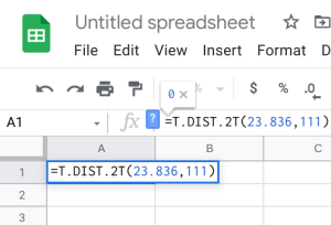
-
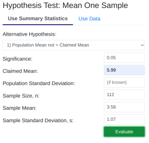
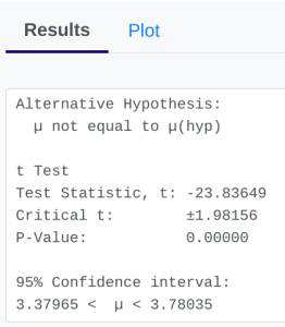
- StatDisk: We can conduct this test using StatDisk. The nice thing about StatDisk is that it will also compute the test statistic. From the main menu above we click on Analysis, Hypothesis Testing, and then Mean One Sample. From there enter the 0.05 significance, along with the specific values as outlined in the picture below in Step 2. Notice the alternative hypothesis is the not = option. The Claimed Mean is [latex]\mu[/latex], the Sample Size is [latex]n[/latex], the Sample Mean is [latex]\bar{x}[/latex], and the Sample Standard Deviation is [latex]s[/latex], then click on Evaluate. If you check the values, the test statistic is reported in the Step 3 display, as well as the P-Value of [latex]0.000[/latex].
-
Step 1 Step 2 Step 3 
-
- Microsoft Excel: You don’t need to have the Data Analysis ToolPack installed for this. We can use the built-in T.DIST.2T function to help calculate it. The function will be typed into an empty cell in Excel (either installed on your computer, or using the online version) as =T.DIST.2T(x,deg_freedom), where x is the [latex]t[/latex] test statistic we just calculated (but always entered as a positive value), and deg_freedom is the [latex]df[/latex] we calculated earlier. We would enter =T.DIST.2T(23.836,111). Notice the 1.81E-45 in the second picture. This is scientific notation; the -45 indicates we move the decimal 45 spaces to the left, which basically leaves a bunch of zeros. This gives us a [latex]p-value[/latex] of [latex]0.000[/latex].
- Applying the Decision Rule: We now compare this to our significance level, which is 0.05. If the p-value is smaller or equal to the alpha level, we have enough evidence for our claim, otherwise we do not. Here, [latex]p-value = 0.000[/latex], which is definitely smaller than [latex]\alpha = 0.05[/latex], so we have enough evidence for the claim…but what does this mean?
- Conclusion: Because our p-value of [latex]0.000[/latex] is less than our [latex]\alpha[/latex] level of [latex]0.05[/latex], we reject [latex]H_{0}[/latex]. We have convincing evidence that the true mean price of a Big Mac in Imperial County is different that prices around the world.
Example 2: Bacteria in Swimming Pools
A random sample of water from 30 different pools in Ohio revealed E. coli bacteria levels averaging [latex]\bar{x} = 1231[/latex] per sample with a standard deviation of [latex]s = 1038[/latex]. Using a significance level of [latex]\alpha = 0.05[/latex], test the claim that the population of pools have a mean coliform bacteria level of more than 400. Is there convincing statistical evidence that the bacteria is higher than expected?
Solution
Since we are being asked for convincing statistical evidence, a hypothesis test should be conducted. In this case, we are dealing with averages or means from one sample or group (pools in Ohio), so we will conduct a Test for 1 Mean, [latex]\sigma[/latex] Unknown.
- [latex]n = 30[/latex]
- [latex]df = n -1 = 30 - 1 = 29[/latex]
- [latex]\bar{x} = 1231[/latex]
- [latex]s = 1038[/latex]
- [latex]\alpha = 0.05[/latex] (we are told to use 0.05 or 5%)
- Null and Alternative Hypothesis: Since the claim is specifically asking if the mean is over 400, that goes along with the alternative hypothesis is that [latex]\mu[/latex] is greater than 400. In our example here, the idea that “nothing is different” would be equivalent to saying that [latex]\mu[/latex] is the same as (equal to) 400.
- [latex]H_{0}: \mu = 400[/latex]
- [latex]H_{A}: \mu > 400[/latex]
- [latex]\mu = 400[/latex] (from the null hypothesis)
- Test Statistic
- [latex]t = \displaystyle \frac{\bar{x} - \mu}{\frac{s}{\sqrt{n}}}\ = \displaystyle \frac{1231 - 1038}{\frac{1038}{\sqrt{30}}} = 4.385[/latex] (generally we round [latex]t[/latex] to 3 places)
- P-Value: Here we will get a little bit of practice using some of the power of Excel, Google Sheets, or StatDisk to give us the P-Value.
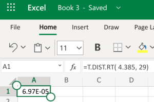
- Microsoft Excel: You don’t need to have the Data Analysis ToolPack installed for this. We can use the built-in T.DIST.RT function to help calculate it. The function will be typed into an empty cell in Excel (either installed on your computer, or using the online version) as =T.DIST.RT(x,deg_freedom), where x is the [latex]t[/latex] test statistic we just calculated (but always entered as a positive value), and deg_freedom is the [latex]df[/latex] we calculated earlier. The “RT” in the formula is for the “more than” problems. Step 1 illustrates how we would enter =T.DIST.RT(4.385,29). Step 2 gives us 6.97E-5, which is in scientific notation; the -5 indicates we move the decimal 5 spaces to the left, which basically leaves several zeros. This gives us a [latex]p-value[/latex] of \(0.000\).
-
Step 1 Step 2 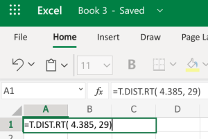
-
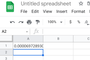
- Google Sheets: You can also do this using the exact same built-in function within Google Sheets. We can use the built-in T.DIST.RT function to help calculate it. The function will be typed into an empty cell in Google Sheets as =T.DIST.RT(x,deg_freedom), where x is the [latex]t[/latex] test statistic we just calculated (but always entered as a positive value), and deg_freedom is the [latex]df[/latex] we calculated earlier. The “RT” in the formula is for the “more than” problems. Step 1 illustrates how we would enter =T.DIST.RT(4.385,29). Step 2 gives us 0.0000697, which gives us a [latex]p-value[/latex] of [latex]0.000[/latex].
-
Step 1 Step 2 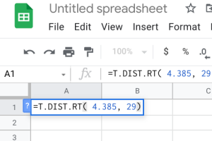
-
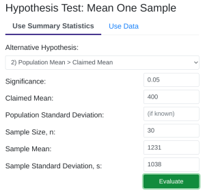
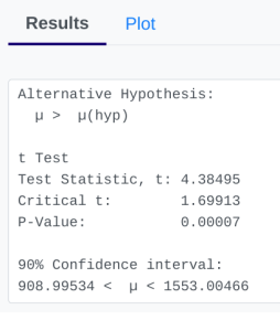
- StatDisk: We can conduct this test using StatDisk. The nice thing about StatDisk is that it will also compute the test statistic. From the main menu above we click on Analysis, Hypothesis Testing, and then Mean One Sample. From there enter the 0.05 significance, along with the specific values as outlined in the picture below in Step 2. Notice the alternative hypothesis is the > option. The Claimed Mean is [latex]\mu[/latex], the Sample Size is [latex]n[/latex], the Sample Mean is [latex]\bar{x}[/latex], and the Sample Standard Deviation is [latex]s[/latex], then click on Evaluate. If you check the values, the test statistic is reported in the Step 3 display, as well as the P-Value of [latex]0.000[/latex] (if we take it to 3 decimal places).
-
Step 1 Step 2 Step 3 
-
- Microsoft Excel: You don’t need to have the Data Analysis ToolPack installed for this. We can use the built-in T.DIST.RT function to help calculate it. The function will be typed into an empty cell in Excel (either installed on your computer, or using the online version) as =T.DIST.RT(x,deg_freedom), where x is the [latex]t[/latex] test statistic we just calculated (but always entered as a positive value), and deg_freedom is the [latex]df[/latex] we calculated earlier. The “RT” in the formula is for the “more than” problems. Step 1 illustrates how we would enter =T.DIST.RT(4.385,29). Step 2 gives us 6.97E-5, which is in scientific notation; the -5 indicates we move the decimal 5 spaces to the left, which basically leaves several zeros. This gives us a [latex]p-value[/latex] of \(0.000\).
- Applying the Decision Rule: We now compare this to our significance level, which is [latex]\alpha = 0.05[/latex]. If the p-value is smaller or equal to the alpha level, we have enough evidence for our claim, otherwise we do not. Here, [latex]p-value = 0.000[/latex], which is definitely smaller than [latex]\alpha = 0.05[/latex], so we have enough evidence for the claim…but what does this mean?
- Conclusion: Because our p-value of [latex]0.000[/latex] is less than our [latex]\alpha[/latex] level of [latex]0.05[/latex], we reject [latex]H_{0}[/latex]. We have convincing evidence that the mean bacteria level is above 400.
Example 3: Are M&M’s Cheating Us Out of Chocolate?
Did you ever notice that sometimes packaged food has a lot of air, or that some items seem smaller than they used to be? The average M&M candy weighs about 1 gram. One day, I got curious and decided to weigh 100 individual M&M candies. The average came out to be [latex]\bar{x} = 0.92[/latex] grams. The standard deviation was [latex]s = 0.03[/latex] grams. Is there convincing statistical evidence that we are being cheated out of M&M chocolate?
Solution
Since we are being asked for convincing statistical evidence, a hypothesis test should be conducted. In this case, we are dealing with averages or means from one sample or group (M&M candies), so we will conduct a Test for 1 Mean, [latex]\sigma[/latex] Unknown.
- [latex]n = 100[/latex]
- [latex]\bar{x} = 0.95[/latex] grams
- [latex]s = 0.03[/latex] grams
- [latex]\alpha = 0.05[/latex] (we were not told a specific value in the problem, so we are assuming it is 5%)
- Null and Alternative Hypothesis: Since the average M&M weighs 1 gram, and the question is whether the we are being cheated out of chocolate, the claim that goes along with the alternative hypothesis is that [latex]\mu[/latex] is less than 1 gram. In our example here, the idea that “nothing is different” would be equivalent to saying that [latex]\mu[/latex] is the same as (equal to) 1 gram.
- [latex]H_{0}: \mu = 1[/latex]
- [latex]H_{A}: \mu < 1[/latex]
- [latex]\mu = 1[/latex] (from the null hypothesis)
- Test Statistic
- [latex]t = \displaystyle \frac{\bar{x} - \mu}{\frac{s}{\sqrt{n}}}\ = \displaystyle \frac{0.95 - 1}{\frac{0.03}{\sqrt{100}}} = -26.667[/latex] (generally we round [latex]t[/latex] to 3 places)
- P-Value: Here we will get a little bit of practice using some of the power of Excel, Google Sheets, or StatDisk to give us the P-Value.
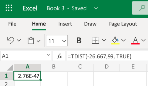
- Microsoft Excel: You don’t need to have the Data Analysis ToolPack installed for this. We can use the built-in T.DIST function to help calculate it. The function will be typed into an empty cell in Excel (either installed on your computer, or using the online version) as =T.DIST(x,deg_freedom,cumulative), where x is the [latex]t[/latex] test statistic we just calculated, and deg_freedom is the [latex]df[/latex] we calculated earlier. We enter “TRUE” for the cumulative portion. Step 1 illustrates how we would enter =T.DIST(-26.667,99,TRUE). Step 2 gives us 2.76E-47, which is in scientific notation; the -47 indicates we move the decimal 47 spaces to the left, which basically leaves a bunch of zeros. This gives us a [latex]p-value[/latex] of [latex]0.000[/latex].
-
Step 1 Step 2 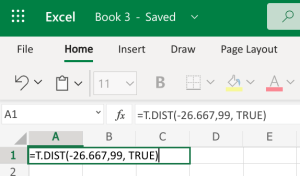
-
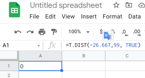
- Google Sheets: You can also do this using the exact same built-in function within Google Sheets. We can use the built-in T.DIST function to help calculate it. The function will be typed into an empty cell in Google Sheets as =T.DIST(x,deg_freedom,cumulative), where x is the [latex]t[/latex] test statistic we just calculated, and deg_freedom is the [latex]df[/latex] we calculated earlier. We enter “TRUE” for the cumulative portion. Step 1 illustrates how we would enter =T.DIST(-26.667,99,TRUE). Step 2 gives us 0, which gives us a [latex]p-value[/latex] of [latex]0.000[/latex].
-
Step 1 Step 2 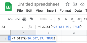
-
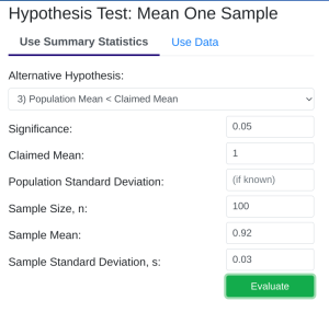
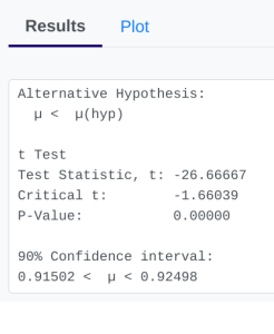
- StatDisk: We can conduct this test using StatDisk. The nice thing about StatDisk is that it will also compute the test statistic. From the main menu above we click on Analysis, Hypothesis Testing, and then Mean One Sample. From there enter the 0.05 significance, along with the specific values as outlined in the picture below in Step 2. Notice the alternative hypothesis is the < option. The Claimed Mean is [latex]\mu[/latex], the Sample Size is [latex]n[/latex], the Sample Mean is [latex]\bar{x}[/latex], and the Sample Standard Deviation is [latex]s[/latex], then click on Evaluate. If you check the values, the test statistic is reported in the Step 3 display, as well as the P-Value of [latex]0.000[/latex] (if we take it to 3 decimal places).
-
Step 1 Step 2 Step 3 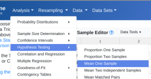
-
- Microsoft Excel: You don’t need to have the Data Analysis ToolPack installed for this. We can use the built-in T.DIST function to help calculate it. The function will be typed into an empty cell in Excel (either installed on your computer, or using the online version) as =T.DIST(x,deg_freedom,cumulative), where x is the [latex]t[/latex] test statistic we just calculated, and deg_freedom is the [latex]df[/latex] we calculated earlier. We enter “TRUE” for the cumulative portion. Step 1 illustrates how we would enter =T.DIST(-26.667,99,TRUE). Step 2 gives us 2.76E-47, which is in scientific notation; the -47 indicates we move the decimal 47 spaces to the left, which basically leaves a bunch of zeros. This gives us a [latex]p-value[/latex] of [latex]0.000[/latex].
- Applying the Decision Rule: We now compare this to our significance level, which is [latex]\alpha = 0.05[/latex]. If the p-value is smaller or equal to the alpha level, we have enough evidence for our claim, otherwise we do not. Here, [latex]p-value = 0.000[/latex], which is definitely smaller than [latex]\alpha = 0.05[/latex], so we have enough evidence for the claim…but what does this mean?
- Conclusion: Because our p-value of [latex]0.000[/latex] is less than our [latex]\alpha[/latex] level of [latex]0.05[/latex], we reject [latex]H_{0}[/latex]. We have convincing evidence that we are being cheated out of M&M’s chocolate!
