Objectives:

We are going to learn:

• How to get equation of motion for single degree of freedom (SDOF) system by: Force Balance and Moment Balance Method.
• How to get equation of motion by Lagrange’s Equation for translational and rotational motion.
• Still finding equivalent mass, stiffness and dissipation. 
• Determine natural frequency, damped frequency, and damping factor of a system.

Force Balance Method (Translating Systems): 

Consider the Principle of Linear Momentum:

[latex]F=\frac{dP}{dt}=\frac {d mv}{dt}= m \frac{dv}{dt}=ma[/latex]

[latex]F-ma=0[/latex]

The sum of the external forces and inertial forces acting on the system is zero.

Force Balance for Horizontal System: 

We need to find the forces acting on the mass by the individual elements (inertia, stiffness and damping):

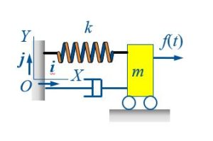
The forces from inertia (i.e., mass), spring and damper are resisting the motion of the mass.

[latex]-kx-c \dot x-m \ddot x+ f(t)=0[/latex]

Equation of Motion: [latex]m \ddot x+c \dot x+ kx =f(t)[/latex]. It should be noted that the solution of the equation of motion (2nd order differential equation) is the displacement of the mass in time ( [latex]x(t)[/latex]).

Force Balance for Vertical System: 

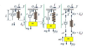
At rest, the static deflection of the spring is due to the weight of the mass. Therefore, we can write: [latex]k \delta_st = mg[/latex]

In motion, by summing up the forces, we get:

[latex]f(t)+mg-k(x+\delta_st)-c \dot x-m \ddot x=0[/latex]

The final equation of motion: [latex]m \ddot x+ c \dot x+ kx=f(t)[/latex]

Force transmitted to Base: 

We consider only the dynamic component of it. By the force transmitted to the base can be written as:

[latex]F_R=k \delta_st+kx+c \frac{dx}{dt}[/latex]

Moment Balance Method (Rotating Systems): 

Principle of angular momentum states that [latex]M= dH/dt=J_G \ddot \theta_k[/latex]

[latex]M-J_G \ddot \theta_k=0[/latex]. By performing moment balance, we will get:

[latex]J_G \ddot \theta + c_t \dot \theta + k_t \theta= M(t)[/latex]

Summary:

Linear single degree of freedom systems are governed by a linear second order ordinary differential equation (ODE) with: *Inertia, *Damping, *Stiffness, and *external force (or moment).

Normalized Governing Equation: 

As shown previously, the typical equation of motion can be written as:

[latex]m \ddot x+c \dot x + k x=f(t)[/latex]

If we divide the above equation by [latex]m[/latex]:

[latex]\ddot x+ \frac{c}{m} \dot x+ \frac{k}{m} x=\frac{f(t)}{m}[/latex]

Then we can get to the some terminologies:

[latex]\omega_n=\frac{k}{m}[/latex] which is defined as the natural frequency.

[latex]2 \zeta=\frac{c}{m \omega_n}[/latex]

Therefore the equation of motion can be written as:

[latex]\ddot x+2 \zeta \omega_n \dot x+ (\omega_n)^2=\frac{f(t)}{m}[/latex]

Natural frequency for translation osciilations for SDOF systems can be defined as: [latex]\omega_n=2 \pi f_n=\sqrt(k/m)[/latex]

where [latex]f_n[/latex] is also the natural frequency expresessed in Hertz (Hz =1/s).

For a system that oscillated along the vertical direction, since [latex]k \delta_st=mg[/latex], we can solve for [latex]k/m=g/\delta_st[/latex]. So, [latex]\omega_n=\sqrt(g/\delta_st)[/latex].

Damping factor ([latex]\zeta[/latex]) is dimensionless. In Chapter 4, we will investigate the effect of different values of damping factor on the response of the system and its vibration, however, for now please note the following definitions:

1. If [latex]\zeta0[/latex], the system is known as undamped.
2. If [latex]0<\zeta<1[/latex], the system is known as underdamped.
3. If [latex]\zeta=1[/latex], the system is known as critically damped. 
4. If [latex]\zeta>1[/latex], the system is known as over-damped.

Please note that all of the above definitions hold for either translational or rotational oscillations. The major difference would be the fact that the units of the equation of motion of a system that is going through translations will be in Force [N or lbs.] whereas for the rotational oscillation, it will be in moments [N.m. or lbs.ft].

In this section of the Chapter, we would like to consider two specific case studies and learn how to develop the equation of motion for these systems: (1) Systems with base excitation, and (2) Systems with unbalanced rotating masses.

Systems with Base Excitation: 

Find the equation of motion of the package on the truck. Assume the displacement is only vertical.

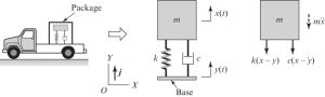
By performing the force balance method and inspecting the free body diagram on the right side of Figure 3-3, we can write the equation of motion as below:

[latex]m \ddotx+ c (\dot x -\dot y)+k (x-y)=0[/latex]

If we move the terms associated with the base movement (y(t)) to the right hand side of the equation, we get:

[latex]m \ddotx+ c (\dot x)+k (x)= k (y)+ c (\dot y)[/latex]

It should be noted that the general form of the equation of motion is the same, the base movement is acting as an excitation force when it is moved to the right hand side. In Chapter 5 and 6, we will learn how we can solve the equation of motion if there is a forcing term on the right hand side.

Systems with Unbalanced Rotating Mass: 

Find the equation of motion of the system shown below. Assume the displacement of the mass M is only vertical.

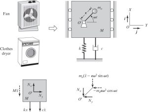
The forces shown on Figure 3-4 are the reaction forces that will be applied to the point O’ due to rotation of pendulum [latex]m_0[/latex]. By performing a force balance in the vertical direction (X axis in this case), we will get:

[latex]M \ddot x+ kx+ c \dotx + m_0 (\ddot x - \epsilon \omega^2 sin \omega t)=0[/latex]

If we re-arrange the terms, we get:

[latex](M+m_0) \ddot x+ kx+ c \dotx = m_0 ( \epsilon \omega^2 sin \omega t)[/latex]

[latex]\ddot x+ 2\zeta \omega_n \dot x+ (\omega_n)^2 x= \frac{F(\omega)}{m} sin \omega t[/latex]

where [latex]m=M+m_0[/latex], [latex]\omega_n=\sqrt (k/m)[/latex], and [latex]F(\omega)=m_0 \epsilon \omega^2[/latex].

Lagrange’s Equation Method:

Let us consider a system of N degrees of freedom that is described by a set of N generalized coordinates: [latex]q_i[/latex] for [latex]i=1, 2, 3, ...[/latex].

These coordinates are unconstrained, independent coordinates, that is , they are not related to each other by geometrical or kinematical conditions.

Recall: Degreee of freedom is defined as the minimum number of generalized coordinates needed to describe a system. 

Lagrange’s equations have the general form of:

[latex]\frac{d}{dt} (\frac {\partial T}{\partial \dot q_j})-\frac{\partial T}{\partial q_j}+\frac{\partial D}{\partial \dot q_j}+\frac {\partial V}{\partial q_j}=Q_j[/latex]

where [latex]\dot q_j[/latex]: generalized velocities

[latex]T[/latex]: Kinetic Energy

[latex]D[/latex]: Dissipation Energy

[latex]V[/latex]: Potential Energy

and [latex]Q[/latex]: Generelized Force/Moment.

Example: Find the equation of motion of the system shown below by using Lagrange’s Equation.

The mass [latex]m_1 and m_2[/latex] are going through the rotational motion and are rotating about point O.

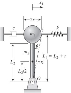
First we find the total kinetic energy (T):

[latex]J_o=J_o1+J_o2[/latex]

[latex]J_o1= 2/5 m_1 r^2 + m_1 (L_1)^2=m_1 (2/5 r^2+(L_1)^2)[/latex]

[latex]J_o2=1/12 m_2 (L_2)^2+m_2 (L_2/2)^2=1/3 m_2 (L_2)^2[/latex]

The total kinetic energy: [latex]T=\frac{1}{2} J_o \dot \theta^2=\frac{1}{2}[m_1(\frac{2}{5}r^2[/latex]+L_1^2)+\frac{1}{3}m_2 L_2^2]\dot \theta^2

Since we are assuming small angle oscillations, we can write [latex]x_1=L_1 \theta_1[/latex].

The total potential energy will include the potential energy of spring K1, gravitational potential energy of the two masses:

[latex]V_1=\frac{1}{2}k x_1^2=\frac{1}{2}(kL_1^2)\theta^2[/latex]

[latex]V_2+V_3=\frac{1}{2}m_1gL_1 \theta^2+ \frac{1}{2} m_2 g L_2/2 \theta^2[/latex]

[latex]V_total=V_1+V_2+V_3=\frac{1}{2}[kL_1 ^2 -m_1 g L_1 -m_2 g L_2/2] \theta^2[/latex]

The total dissipation energy is: [latex]D=\frac{1}{2} c \dot (x_1)^2=\frac{1}{2} (cL_1^2)\dot \theta^2[/latex]

Then we perform the Lagrange’s equation operation to get the equivalent mass, damping, and stiffness to form the equation of motion.