OBJECTIVES
We will learn, how to:
- Determine the solutions for a linear, single DOF system that is undamped, critically damped, over-damped, and undamped.
- Determine the response of single DOF systems to initial conditions (ICs) and use the results to study the reponse of impacts and collisions.
The topic that will be covered in this chapter are as follows:
- Free responses and characteristics for different damping scenarios
- State-space plots (phase portrait plots)
- Displacement and velocity extrema
- Logarithmic decrement
- Laplace transfrom
- Stability for free oscillations
FREE RESPONSE
In previous chapter, we have learned how to find the equation of motion of a SDOF system that is experiencing external forces. In this chapter, we will learn how to solve that equation of motion for a special case of non-forcing system (i.e. there will be no external force applied to the system). In these systems, the right hand side of the equation of motion equals zero (i.e., [latex]f_ext (t)=0[/latex]0.
Therefore for a system shown below, we are tasked to find [latex]x(t)[/latex] for a given initial displacement [latex]x(0)=X_0[/latex] and initial velocity [latex]\dot x(0)=V_0[/latex]. The response of a system to initial conditions [latex]X_0[/latex]and [latex]V_0[/latex] is called Free Response.
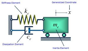
We know the equation of motion will be [latex]\ddot x+2 \zeta \omega_n \dot x+ (\omega_n)^2=\frac{f(t)}{m}[/latex]. When [latex]f(t)=0[/latex] (no forcing term), the response of undamped and damped system is called free response. Before getting the solutions to this equation of motion, we need to understand two major concepts: 1) Period of Undamped Free Oscillation and 2) Period of Damped Free Oscillation.
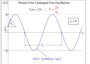
For an undamped system under free oscillations, the system (theoretically) will be oscillating at a constant frequency, equal to its natural frequency [latex]\omega_n[/latex], with a fixed and constant oscillation amplitude. Figure 4-2 represents this form of oscillation. It should be noted that the system shown below experiences both initial displacement ([latex]X_0[/latex]) and initial velocity ([latex]V_0[/latex]). The oscillation can be written in terms of a sinusoidal function shown in the graph.
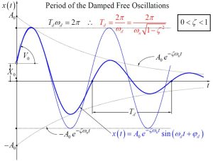
For a damped system under free oscillation, there is an exponential decay to the oscillation as times continues. Therefore, the oscillation is bounded by a negative exponential function. Additionally, the frequency of oscillation is no more equal to natural frequency but is equation to damped natural frequency which is equal to [latex]\omega_n \sqrt{(1-\zeta^2)}[/latex]. Figure below represents a damped free oscillation system.
The following table represents a list of solutions for different damping scenarios:
| Type of Damping | [latex]\zeta[/latex] Value | Solution |
| Undamped | [latex]\zeta=0[/latex] | [latex]x(t)=X_0 cos (\omega_n t)+\frac {V_0}{\omega_n} sin (\omega_n t)[/latex] |
| Underdamped | [latex]0<\zeta<1[/latex] | [latex]x(t)=X_0 e^{(-\zeta \omega_n t)} cos (\omega_d t)+ \frac{V_0 +\zeta \omega_n X_0}{\omega_d} e^{ (-\zeta \omega_n t)} sin (\omega_d t)[/latex] |
| Critically Damped | [latex]\zeta=1[/latex] | [latex]x(t)=X_0 e^{(- \omega_n t)}+[V_0+ \omega_n X_0] t e^{-\omega_n t}[/latex] |
| Over-damped | [latex]\zeta>1[/latex] | [latex]x(t)=X_0 e^{-\zeta \omega_n t} cosh(\omega_d' t)+ \frac{V_0+\zeta \omega_n X_0}{\omega_d'}e^(-\zeta \omega_n t) sinh (\omega_d' t)[/latex] where [latex]\omega_d'=\omega_n \sqrt{\zeta^2 -1}[/latex] |
State Space Plots
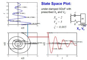
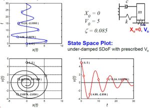
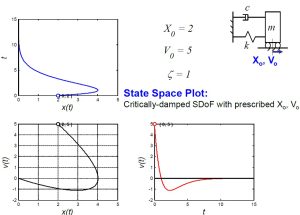
These plots are usually made of three portions: (1) Top-Left Corner: This graph is the response of the system (displacement) over time. It is graphed with time (in seconds) in vertical axis and displacement (x(t)) in horizontal axis.(2) Bottom-Left Corner: This graph is velocity versus displacement and (3) Bottom-Right Corner: Velocity versus time.
1) [latex]X_0=2, V_0=5, and \zeta=0.085[/latex]: For a SDOF underdamped system with initial displacement of [latex]X_0=2[/latex] and [latex]V_0=5[/latex] with the damping ratio of [latex]\zeta=0.085[/latex]. the state space plot will look as shown below.
2) [latex]X_0=0, V_0=5, and \zeta=0.085[/latex]: For a SDOF underdamped system with initial displacement of [latex]X_0=0[/latex] and [latex]V_0=5[/latex] with the damping ratio of [latex]\zeta=0.085[/latex]. the state space plot will look as shown below.
3) [latex]X_0=2, V_0=5, and \zeta=1[/latex]: For a SDOF critically damped system with initial displacement of [latex]X_0=2[/latex] and [latex]V_0=5[/latex] with the damping ratio of [latex]\zeta=1[/latex]. the state space plot will look as shown below.
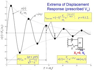
Extrema of Displacement Response (prescribed [latex]V_0[/latex]
In order to find the maximum and minimum points in the displacement response, the first derivative with respect to time is taken and set equal to zero. This equation is then solved for time. The displacement has an extremum (max or min) at those times [latex]t_dm[/latex]. Lets recall that the displacement function for an underdamped system that has zero initial displacement looks as shown below:
[latex]x(t)=\frac{V_0}{\omega_d}e^(-\zeta \omega_n t)sin(\omega_d t)[/latex]
If we take the derivative: [latex]\dot x(t_dm)=-\frac{V_0}{\sqrt{(1-\zeta^2)}}e^{-zeta \omega_n t_dm} sin(\omega_d t_dm-\phi)=0[/latex]
Solution to the above equation will be: [latex]sin(\omega_d t_dm -\phi)=0[/latex] and then [latex]\omega_d t_dm=\phi + p \pi[/latex] for p=0, 1, 2, … , where [latex]\phi=tan^{-1} (\sqrt{1-\zeta^2}/\zeta)[/latex].
Now, if we plug the above finding into the displacement function, we can find the maximum or minimum displacement value:
[latex]x_max/min=(-1)^p \fract{V_0}{\omega_n}} e^(\frac{\phi+p \pi}{tan \phi})[/latex] for p=0, 1, 2, … .
The following figure represents the summary of these results:
Logarithmic Decrement
The logarithmic decrement [latex]\delta[/latex] can provide useful information in regard to the damping ratio of an underdamped system. In an underdamped system, the system oscillation is bounded by exponential decay. Therefore, the ratio of any corresponding point within the periods is going to be equal to each other. Therefore, one can find the damping factor [latex]\zeta[/latex] from the decrement rate. One can also find the natural frequency, initial conditions from the displacement plots.
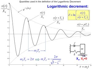
From these two amplitudes, it is possible to determine the damping ratio [latex]\zeta[/latex]. The displacement of the p-th point can be written as: [latex]x_p =x(t+pT_d),[/latex] where p=0, 1, 2, … . By definition of exponential decay,
[latex]e^{\delta}=x_0/x_1=x_1/x_2=x_2/x_3=x_3/x_4=...=x_(p-1)/x_p[/latex].
Now, if we are looking for the ratio of the points [latex]x_0[/latex] and [latex]x_p[/latex], then we can write:
[latex]x_0/x_p=x_0/x_1 x_1/x_2 x_2/x_3 ...x_(p-1)/x_p=e^{\delta} e^{\delta} e^{\delta} ... e^{\delta}=e^{p \delta}[/latex]
So if take natural log of both sides, we can get to the following equation:
[latex]\delta=\frac{1}{p} ln(x_0/x_p)[/latex] where p=0, 1, 2, 3, … .
If you simplify the terms, you will get to the following two equations:
[latex]\delta=\frac{2 \pi \zeta}{\sqrt{1-\zeta^2}}[/latex]
and
[latex]\zeta=\frac{1}{\sqrt{1+(2\pi/\delta)^2}}[/latex]
Laplace Transform
Laplace transform is a useful tool to solve differential equations. It converts the equation of motion (i.e. differential equation) which is in the physical domain (time), to an algebraic equation (in s domain). For an equation of motion, we have a 2nd order linear ODE:
[latex]m \ddot x(t)+c \dot x(t)+ kx(t)=f(t)[/latex]
The Laplace transform is a one-to-one transformation.
Let’s assume we have the above equation of motion, in order to solve the displacement response, one needs to take the laplace of each side of the equation.
Based on the definition of Laplace Transform that is discussed in class, we can find the laplace of individual terms as shown below:
[latex]L{x(t)}=X(s)[/latex]
[latex]L{\dot x(t)}=-x(0)+s X(s)[/latex]
[latex]L{\\dot x(t)}=-\dot x(0)-s x(0)+ s^2 X(s)=-V_0-sX_0+s^2 X(s)[/latex]
Therefore, the Laplace form of EOM will be:
[latex][-V_0-s X_0 +s^2 X(s)]+2 \zeta \omega_n [-X_0 +s X(s)]+ \omega_n^2 X(s)= \fract {1}{m} F(s)[/latex]
[latex]X(s) [s^2+ 2\zeta \omega_n s+ \omega_n ^2]+[-s X_0]+[-V_0 - 2\zeta \omega_n X_0]=\frac{1}{m}F(s)[/latex]
Let us define [latex]D(s)=[s^2 + 2 \zeta \omega_n s+ \omega_n^2][/latex]
So if we solve for [latex]X(s)[/latex]:
[latex]X(s)=\frac{s X_0}{D(s)}+\frac {(V_0+2\zeta \omega_n X_0)}{D(s)}+ \frac{1}{m} \frac{F(s)}{D(s)}[/latex]
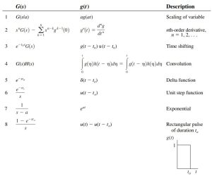
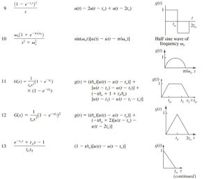
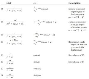
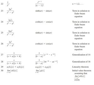
By going back to the Laplace Transformation table, Pairs 14, 16 and 4 can be used to find the Laplace Inverse functions in time domains:
Pair 14: [latex]L^-1{\frac{1}{s^2+2\zeta \omega_n s+ \omega_n^2}}=\frac{1}{\omega_d} e^(-zeta \omega_n t) sin (\omega_d t)[/latex]
Pair 16: [latex]L^-1{\frac{2}{s^2+2\zeta \omega_n s+ \omega_n^2}}=\frac{\omega_n}{\omega_d} e^(-zeta \omega_n t) sin (\omega_d t-\phi)[/latex]
Pair 4: [latex]Convolution Integral[/latex]