Objectives:
In this chapter, we are going to:
- Review some basics of linear algebra and vector operations.
- Determine the displacement, velocity and acceleration of a mass element.
- Determine the number of degrees of freedom of a system.
- Determine the linear momentum and angular momentum of a rigid body.
- Determine the kinetic energy and the work of a system.
Linear Algebra:
- Matrix is a rectangular array of quantities as shown below:
[latex][A]=\begin{bmatrix}
a_{11} & a_{12} & \dots & a_{1n}\\
a_{21} & a_{22} & \dots & a_{2n}\\
\vdots &\vdots &\ddots & \vdots\\
a_{m1} & a_{m2}&....&a_{mn}
\end{bmatrix}[/latex]
The above matrix would be called a “square matrix” if m=n.
By definition, the transpose of a matrix is also defined as:
[latex][A]^T=\begin{bmatrix}
a_{11} & a_{21} & \dots & a_{m1}\\
a_{12} & a_{22} & \dots & a_{m2}\\
\vdots &\vdots &\ddots & \vdots\\
a_{1n} & a_{2n}&....&a_{mn}
\end{bmatrix}[/latex]
Note that the diagonal terms in a matrix and its transpose are the same and do not change. Additionally, a symmetric matrix is defined by: [latex]$[A]=[A]^T[/latex] and a skew-symmetric matrix is defined by: [latex]$[A]=-[A]^T[/latex].
- Column matrix (Column vector) is a matrix that has only one column and looks as shown:
[latex][a]=\begin{bmatrix}
a_{11} \\
a_{21}\\
\vdots\\
a_{m1}\\
\end{bmatrix}=\begin{bmatrix}
a_{1}\\
a_{2}\\
\vdots\\
a_{m}\\
\end{bmatrix}[/latex]
- Row matrix (Row vector) is a matrix that has only one row and looks as shown:
[latex][a]^T=\begin{bmatrix}=a_{1}&a_{2}&\dots&a_{m}\end{bmatrix}[/latex]
Note that the dimensions of the column matrix {a} are m×1 while the dimensions of the row matrix {a}T are 1×m .
- Diagonal Matrix is a matrix that its off-diagonal terms are zero:
[latex]
[A]=\begin{bmatrix}
a_{11} & 0 & \dots & 0\\
0& a_{22} & \dots &0\\
\vdots &\dots &\ddots & \vdots\\
0 & 0&....&a_{mn}
\end{bmatrix}
[/latex]
- Identity Matrix is a diagonal matrix that its diagonal entries are all one:
[latex]
[A]=\begin{bmatrix}
1 & 0 & \dots & 0\\
0 & 1& \dots &0\\
\vdots &\dots &\ddots & \vdots\\
0 & 0&....&1
\end{bmatrix}
[/latex]
- Determinant of a Square (3×3) Matrix: Determinant, in linear algebra, is a value denoted by [latex]$det[A]$[/latex], associated with a square matrix [latex]$[A]$[/latex] of n rows and n columns. If we are given the following 3 by 3 matrix:
[latex][A]=\begin{bmatrix}=
a_{11}&a_{12}&a_{13}\\
a_{21}&a_{22}&a_{23}\\
a_{31}&a_{32}&a_{33}\\
\end{bmatrix}
[/latex]
Then we can define its determinant as:
[latex]\begin{aligned}Det[A]=
&a_{11}[(a_{22}\times&a_{33})-(a_{23}\times&a_{32})]\\
&-a_{12}[(a_{21}\times&a_{33})-(a_{23}\times&a_{31})]\\
& a_{13}[(a_{21}\times&a_{32})-(a_{22}\times&a_{31})]\end{aligned}[/latex]
A matrix is called a “singular” matrix if [latex]$Det[A]=0$[/latex].
- Addition and Subtraction of Matrices:
[latex][C]=[A]\pm[B]\\ c_{ij}=a_{ij}\pm&b_{ij}[/latex] for every i and j.
- Multipication of Matrices:
[latex][C]=[A][B]\\ c_{ij}=\sum&a_{ip}b_{pj}[/latex] for p values from 1 to k.
- Useful Properties of Matrix Products: The following provides some useful properties in matrix operations to consider in Linear Algebra:
[latex][A][B]&\neq&[B][A]\\ ([A][B])^T=[B]^T[A]^T [C]([A][B])=([C][A])[B] ([A] [B])[C]=[A][C] [B][C][/latex]
- Inverse of a square matrix has the following unique property: [latex]$[A]^{-1}[A]=[A][A]^{-1}=[I]$[/latex].
- If and only if [latex]$[A]$[/latex] is not singular; i.e. [latex]&det[A]&\neq&0&[/latex], ‘Eigen Values of a square matrix and roots of the characteristic equation can be found by:
[latex]$det[[A]-\lambda[I]]=0$[/latex]
NOTE: Matrix of order n has n eigenvalues.
Dynamics:
- Scalar Quantity has a magnitude without direction. For example, mass, temperature, energy or speed are all scalar quantities.
- Vector Quantity has magnitude and direction. For example, position, velocity, acceleration, force, linear momentum are all vector quantities.
- A vector quantity can be written in form of a column or row matrix. This is where Linear Algebra can become helpful in performing different mathematical operations on different physical vector quantities.
- For example, the following vector in 3D coordinate system can be written as shown:
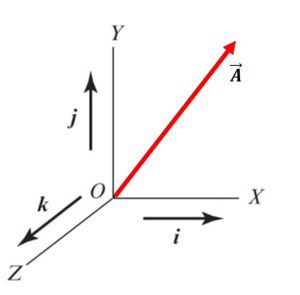
[latex]$\vec{A}=\vec{A_{x}} \vec{A_{y}} \vec{A_{z}}=A_{x}i A_{y}j A_{z}k$[/latex].
- Vector Algebra:
- Vector addition is both commutative and associative. Therefore the following relationships hold:
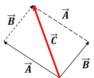
Figure 1-2: Vector Addition [latex]C=A B=B A[/latex]
[latex](A B) C=A (B C)[/latex]
- Vector Subtraction:
- Vector addition is both commutative and associative. Therefore the following relationships hold:
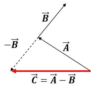
[latex]A-B=A (-B)[/latex]
-
- Vector Products:
(1) Scalar Dot Product: The dot product is one way of multiplying two or more vectors. Algebraically, it is the sum of the products of the corresponding entries of two sequences of numbers. Geometrically, it is the product of the Euclidean magnitude of two vectors and the cosine of the angle between them.
Assuming the angle between the two vectors A and B is [latex]$\theta$[/latex], the dot product between them is defined as:
[latex]A.B=A.B.Cos\theta[/latex]
It should be noted that the result of a dot product is always a scalar quantity. Additionally, it is important to understand that [latex]A.B=B.A[/latex]. Based on the above definitions, in order to find if two vectors are perpendicular (i.e. angle between them is 90 degrees), one can perform a dot product since:
[latex]If&\theta=90&, A.B=0[/latex].
Additionally, a dot product is known as the summation of the products of conjugates. Mathematically, this can be represented as the following:
Assume, we have a vector [latex]\vec{A}=(A_{x}i A_{y}j A_{k}z)[/latex] and another one is [latex]\vec{B}=(B_{x}i B_{y}j B_{k}z)[/latex], the dot product of the two vectors can be found as shown below:
[latex]A.B=(A_{x}i A_{y}j A_{k}z).(B_{x}i B_{y}j B_{k}z)= A_{x}B_{x} A_{y}B_{y} A_{z}B_{z}.[/latex]
(2) Vector Cross Product: Given two linearly independent vectors a and b, the cross product is a vector that is perpendicular to both of the vector and thus normal to the plane containing them. By definition, the cross product of the two vectors A and B mentioned above, can be written as:
[latex]C=A\times&B=|A| |B| Sin \theta= B \times A=-A \times B[/latex]
It should also be noted for the cross product of unit vectors i, j, and k:
[latex]i \times j =k[/latex]
[latex]j \times k =i[/latex]
[latex]k \times i=j[/latex]
If the angle between them is zero, the cross product will also be zero since the sine of the angle zero is equal to zero.
Kinematics of Particles and Rigid Bodies
- Unit vectors i, j, and k are fixed in the reference frame R. The unit vectors i, j, and k are orthogonal with each other and fixed in time.
- Point O is the origin of the XYZ coordinate system.
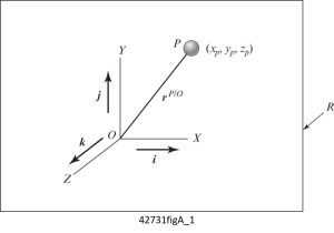
Figure 1-4: Kinematics of Particle Position Vector [latex]\vec{r}^{P/O}=\vec{r}=\vec{x}_p(t)i \vec{y}_p(t)j \vec{z}_p(t)k[/latex] Velocity Vector [latex]\vec{v}^{P/O}=\frac{d\vec{r}}{dt}=\dot{\vec{x}}_p(t)i \dot{\vec{y}}_p(t)j \dot{\vec{z}}_p(t)k[/latex] Acceleration Vector [latex]\vec{a}^{P/O}=\frac{d\vec{x}}{dt}=\ddot{\vec{x}}_p(t)i \ddot{\vec{y}}_p(t)j \ddot{\vec{z}}_p(t)k[/latex] - R is called an “inertial reference frame.”:
- An inertial reference frame is stationary and does not have any of the motions of the particles or bodies considered in vibration or dynamic problems.
- The velocity and acceleration defined with respect to a fixed point O in an inertial reference frame R are referred to as the absolute velocity and absolute acceleration.
- In contrast, sometimes we may deal with relative velocity and relative acceleration defined relative to another moving point in R. This will be discussed later in this chapter.
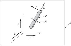
Planar Rigid-Body Kinematics
In Figure 1-5, a rigid-body is going through a planar motion in X and Y plane:
- i, j, and k are fixed in reference frame R and in time.
- [latex]e_1[/latex] and [latex]e_2[/latex] are fixed in reference frame [latex]R'[/latex] (fixed to the body).
- [latex]e_1[/latex] and [latex]e_2[/latex] are defined in the XY plane. Thus, their vector cross product is: [latex]e_1 \times e_2=k[/latex].
- It should be noted that unit vectors [latex]e_1[/latex] and [latex]e_2[/latex] share the motion of the body and change with respect to time.
- General motion of this rigid body can be decomposed into:
- Translation of the center of mass (G)
- Rotation about point (G).
Position, Velocity and Acceleration of the Center of Mass:
We assume it is a single point on a body:
| Position Vector | [latex]\vec{r}^{G/O}=\vec{r}=\vec{x}_G(t)i \vec{y}_G(t)j[/latex] |
| Velocity Vector | [latex]\vec{v}^{G/O}=\frac{d\vec{r}}{dt}=\dot{\vec{x}}_G(t)i \dot{\vec{y}}_G(t)j[/latex] |
| Acceleration Vector | [latex]\vec{a}^{G/O}=\frac{d\vec{v}}{dt}=\ddot{\vec{x}}_G(t)i \ddot{\vec{y}}_G(t)j[/latex] |
Velocity and Acceleration of any other point P on the body:
Let [latex]\omega[/latex] be the angular velocity of the rigid body and [latex]\alpha[/latex] be the angular acceleration of the rigid body.
In addition, we have that:
[latex]d(e_1)/dt=\omega \times e_1[/latex] and [latex]d(e_2)/dt=\omega \times e_2[/latex]
The derivation starts by defining the position vector for the point on the body with respect to the origin of the coordinate system O:
[latex]r^{P/O}=r^{G/O} r^{P/G}[/latex]
[latex]r^{P/O}=r^{G/O} |r^{P/G}|e^1[/latex] where [latex]|r^{P/G}|[/latex] is scalar.
To get the velocity vector, the time derivative will be:
[latex]v^{P/O}=dr^{G/O}/dt d(e_1 r^{P/G})[/latex]
[latex]=v^{G/O} \omega \times e_1 |r^{P/G}|= v^{G/O} \omega \times r^{P/G}[/latex]
We also note that
[latex]v^{P/O}=v^{G/O} v^{P/G}[/latex] and [latex]v^{P/G}=\omega \times r^{P/G}[/latex]
In order to find the acceleration, we find the second time derivative of displacement vector or first time derivative of velocity vector:
[latex]a^{P/O}=dv^{G/O}/dt d (\omega \times r^{P/G})/dt =a^{G/O} \omega \times dr^{P/G}/dt d\omega/dt .\times r^{P/G} =a^{G/O} \omega \times v^{P/G} \alpha \times r^{P/G}[/latex]
Example 1: Kinematics of a planar pendulum:
We shall determine the velocity and acceleration of the planar pendulum [latex]P[/latex] with respect to point [latex]O[/latex] when it rotates with an angular velocity of [latex]\dot \theta[/latex]. Thus: [latex]\omega=\dot \theta k[/latex].
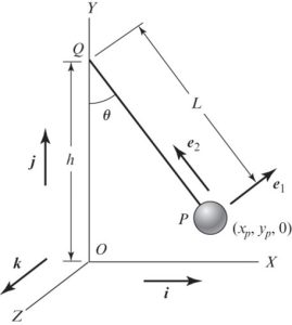
We need to first find the Position Vector. This can be found by following the path from the origin (0,0,0) where the coordinates are fully defined and are fixed in time.
Position Vector:
[latex]r^{P/O}=r^{Q/O} r^{P/Q}=hj-Le_2[/latex]
Velocity Vector: It can be found by taking the time derivative of the position vector:
[latex]v^{P/O}=dr^{P/O}/dt=d (hj-Le_2)/dt =-L de_2/dt= -L (\omega \times e_2)[/latex]
[latex]v^{P/O}=-L(\dot \theta k \times e_2)=L \dot \theta e_1[/latex]
Acceleration Vector:
[latex]a^{P/O}=dv^{P/O}/dt=d (L \dot \theta e_1)/dt[/latex]
[latex]=L \ddot \theta e_1 L \dot \theta de_1/dt[/latex]
[latex]= L \\dot \theta e_1 L \theta \dot \omega \times e_1[/latex]
[latex]=L \ddot \theta e_1+L \dot \theta (\dot \theta k \times e_1)[/latex]
[latex]=L \ddot \theta e_1+L \dot \theta^2 e_2[/latex]
where the first term is the tangential component and the second term is the radial component.
The unit vectors [latex]e_1[/latex] and [latex]e_2[/latex] are resolved in terms of the unit vectors [latex]i[/latex] and [latex]j[/latex] as follows:
Firstly, [latex]e_1=cos \theta i+ sin \theta j[/latex]
Secondly, [latex]e_2=-sin \theta i+ cos \theta j[/latex]
Velocity: [latex]v^{P/O}=L \dot\theta e_1=L \dot \theta (cos \theta i + sin \theta j)[/latex]
Acceleration: [latex]a^{P/O}=L \ddot \theta e_1 + L \dot \theta^2 e_2[/latex]
[latex]=L \ddot \theta (cos \theta i + sin \theta j)+ L \dot \theta^2 (-sin \theta i +cos \theta j)[/latex]
[latex](L \ddot \theta cos \theta - L \dot \theta Sin \theta)i+(L \ddot \theta sin \theta + L \dot \theta^2 cos\theta)j[/latex]
We also note for future use that:
[latex]r^{P/O}=r^{Q/O}+r^{P/Q}=hj-L e_2[/latex]
[latex]=hj -L(-sin \theta i + cos \theta j)[/latex]
If we put the i-terms and j-terms together, we get: [latex](L sin\theta)i+(h-L cos\theta)j[/latex]. Based on this, we can say [latex]P(x,y)=P(L sin\theta, h-L cos \theta)[/latex].
Generalized Coordinates and Degrees of Freedom:
To describe the physical motion of a system, a set of coordinates is required. These coordinates are called generalized coordinates and are commonly represented by the symbol [latex]q_k[/latex]. The generalized coordinates form the smallest possible number of coordinates needed to describe a system.
Additionally, the minimum number of independent coordinates needed to describe the motion of a system is called the degrees of freedom of a system.
The following provides some examples of different systems and their degrees of freedom (DOF):
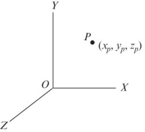
For Example Figure 1-7 requires at least 3 generalized coordinate systems to fully describe the motion of the particle (P): [latex]q_1(t)=x_p(t)[/latex], [latex]q_2(t)=y_p(t)[/latex] and [latex]q_3(t)=z_p(t)[/latex]. Therefore the Figure 1-7 shows a system that has 3 DOFs.
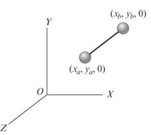
This system is planar, therefore, the z components of each of the end spheres are zero. We have four generalized coordinates left: [latex]q_1=x_a, q_2=y_a, q_3=x_b, and q_4=y_b.[/latex]. If the length of the attachement is known to be L, then, we can write a relationship that makes one of the generalized coordinates be dependent on the other three (i.e., [latex]L=\sqrt((x_a-x_b)^2+(y_a-y_b)^2)[/latex]. Hence, the DOF is three.
Rigid Body Dynamics:
Principle of Linear Momentum: In an inertial reference frame, the rate of change of the linear momentum of a system is equal to the total force acting on this system:
[latex]F=dP/dt[/latex]
where F: total force vector,
P: total linear momentum
d/dt: time derivation.
For a system whose center of mass [latex]m[/latex] is located at a point [latex]G[/latex] and the absolute velocity of this point is [latex]v_G[/latex]; then:
[latex]p=m v_G[/latex]
Based on the above definition, [latex]F=d(mv_G)/dt[/latex]. Based on this definition, we derive the second Newton’s Law of motion: [latex]F=m a_G.[/latex].
Principle of Angular Momentum:
The rate of change of the angular momentum of a system with respect to its center of mass or fixed point is equal to the total moment about this point:
[latex]\mathcal{M}= \frac {d \mathcal{H}}{dt}[/latex]
- [latex]\mathcal{M}[/latex] is net moment acting about a fixed point in the inertial reference frame or about the center of mass of the system.
- [latex]\mathcal{H}[/latex] is the total angular momentum of the system about this point.
- d/dt is the time derivative with respect to the inertial reference frame.
For a rigid body moving in a plane, the angular momentum about the system’s center of mass is: [latex]\mathcal{H_G}=J_G \dot \theta k[/latex]
For a rigid body moving in a plane, the angular momentum about a fixed point in the body: [latex]\mathcal{H_o}=J_o \dot \theta k[/latex]
Work and Energy:
For a system of N particles, the kinetic energy [latex]T[/latex] is:
[latex]T=1/2 \sum m_k (\frac {dr_k}{dt}. \frac {dr_k}{dt})=[/latex]
[latex]1/2 \sum m_k(\dot r_k . \dot r_k)=1/2 \sum m_k (v_k . v_k)[/latex] where [latex]k[/latex] is from 1 to N.
For a rigid body, the kinetic energy [latex]T[/latex] can be expressed as:
[latex]T=T_translational + T_rotational[/latex]
where [latex]T_translational[/latex] is the kinetic energy associated with translation of the center of mass.
and [latex]T_rotational[/latex] is the kinetic energy associated with rotation about the center of mass of the system.
For a rigid body that is rotating AND translation in a plane, we have the form:
[latex]T=\frac {1}{2} m (v_G . v_G)+\frac {1}{2} J_G \dot \theta^2[/latex]
where the first term is the translational part based on the velocity [latex]v_G[/latex] of the center of mass of the system and the second term is the rotational part based on an axis that passes through the center of mass and is normal to the plane of motion.
For a rigid body rotating in the plane about a fixed point O, the kinetic energy is determined from: [latex]T=\frac {1}{2} J_o \dot \theta^2[/latex]
Work-Energy Theorem:
The work is related to the kinetic energy as follows:
[latex]W_AB=T_B-T_A[/latex] (scalar)
where [latex]W_AB[/latex] is the work done in moving the system from the initial point A to the final point B.
[latex]T_B[/latex] is the kinetic energy of the system at B.
[latex]T_A[/latex] is the kinetic energy of the system at A.
Example 2: Kinetic Energy of a Planar Pendulum
Assume the radius of P<<L, therefore, it can be assumed that rotational kinetic energy about center of gravity is much smaller than the translational kinetic energy of the center of gravity.

We shall determine the kinetic energy of the system. Earlier, we have found the velocity of point P:
[latex]v^{P/O}=\frac {dr^{P/O}}{dt}=\frac {d (hj-Le_2)}{dt}=-L \frac {de_2}{dt}[/latex]
[latex]-L \omega \times e_2=-L \dot \theta k \times e_2=L \dot \theta e_1[/latex]
[latex]T_1=\frac {1}{2} m (L \dot \theta)^2 (e_1 . e_1) =\frac{1}{2} m (L^2 \dot \theta^2)[/latex]
Example 3: Kinetic Energy of a rolling disc
A disc of radius [latex]r[/latex] rolls without slipping in the X-Y plane with a constant velocity of [latex]\dot \theta[/latex]
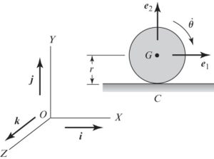
[latex]v^{G/O}=v^{C/O}+v^{G/C}[/latex]
if there is no slipping, that means [latex]v^{C/O}=0[/latex]. Therefore,
[latex]v^{G/O}=v^{G/C}=\omega \times r^{G/C}[/latex]
Also we know [latex]\omega=-\dot \theta k[/latex]. Thus, [latex]v^{G/O}=-\dot \theta k \times rj= r\dot \theta i[/latex]
Kinetic Energy will be:
[latex]T=\frac {1}{2} m(v_G. v_G)+\frac{1}{2} J_G \dot \theta^2= \frac{1}{2} m (\dot \theta r)^2+ \frac {1}{2} J_G \dot \theta^2[/latex]