OBJECTIVES

In Chapter 5, we will learn how to:

• Analyze the responses of SDOF systems to harmonic excitations
• Determine the frequency response and phase of a SDOF
• Interpret the response of a SDOF system for an excitation frequency less than, equal to, and greater than the system’s natural frequency.
• Determine the system parameters from a measured frequency response
• Analyze the responses of a SDOF systems with rotating unbalanced mass and with base excitation

Introduction

In Chapter 4, we learned the response to initial conditions (i.e. initial displacement or initial velocity). In this Chapter, we will learn what is the solution to the equation of motion of a system that is experiencing harmonic excitation as the forcing function.

There are three different systems that we will focus on:

(1) Directly Excited Systems

(2) System with Rotating Unbalanced Mass

(3) System with a moving base (i.e. base excited system)

Response to Harmonic Direct Excitation

Lets recall from Chapter 3, the equation of motion of a directly excited system is as shown below:

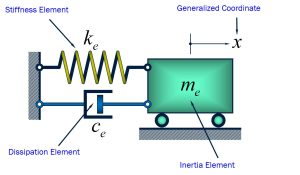
Equation of motion can be written as: [latex]m \ddot x(t)+ c\dotx(t) + k x(t)=f(t)[/latex] where [latex]f(t)=F_0 sin(\omega t)[/latex].

[latex]f(t)[/latex] is a sinusoidal periodic function. Excitation is applied from [latex]t=0[/latex].

CASE 1: Sine Harmonic Excitation:

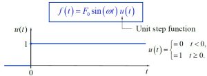
The function can mathematically be defined as:

[latex]f(t)=F_0 sin(\omega t)u(t)[/latex]

The definition of unit step function states that the function is equal to zero for before the time defined and is equal to unity (i.e. 1) for afterwards. The following figure represents the definition of unit step function u(t).

If we have a sinusoidal excitation, the response of the system will be divided into transient and steady state response. Before we get to the solution, we need to define the nondimensional time variable [latex]\tau=\omega_n t[/latex]. Additionally, the Nondimensional excitation frequency is defined as [latex]\Omega=\omega/\omega_n[/latex]. Therefore, if [latex]\Omega=1[/latex], it means excitation frequency is equal to natural frequency.

Based on the above definitions, the overall solution to the given excitation will be defined as shown below:

[latex]x(\tau)=[x_str (\tau)+ x_sss (\tau)] u(\tau)[/latex]

The [latex]x_str[/latex] is defined as transient portion of the solution to sinusoidal solution whereas [latex]x_sss[/latex] is defined as steady-state portion of solution given a sinusoidal excitation.

By performing convolution integral, the steady state portion of the solution can be defined as shown below:

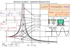
[latex]x_sss (\tau)=\frac{F_0}{k} H(\Omega) sin[\Omega \tau - \theta (\Omega)][/latex].

The coefficient [latex]\frac{F_0}{k}[/latex] is defined as static deflection [latex]\delta_static[/latex]. The amplitude response is defined as shown below:

[latex]H(\Omega)=\frac{1}{\sqrt{D(\Omega)}}=\frac{1}{\sqrt{(1-\Omega^2)^2+(2\zeta \Omega)^2}}[/latex]

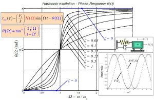
The phase response is defined as following:

[latex]\theta(\Omega)=tan^-1 (\frac{2\zeta \Omega}{1-\Omega^2})[/latex]

The following graph represents the amplitude response as a function of nondimensional excitation frequency for different damping factors. It is shown that as the damping decreases, the peak value of the amplitude response function deviates from being closer to [latex]\Omega=1[/latex]. The peak value for each graph occurs when [latex]\Omega=\sqrt(1-2\zeta^2)[/latex]. This is found by taking the first derivative of [latex]H(\Omega)[/latex] with respect to [latex]\Omega[/latex] and setting it equal to zero and solving for [latex]\Omega[/latex].

The maximum value of amplitude response is equal to [latex]H_max=\frac{1}{2\zeta \sqrt(1-\zeta^2)}[/latex]for [latex]\zeta<\frac{1}{\sqrt(2)}[/latex].

The phase response is also shown in the following graph. It can be seen that when the excitation frequency is equal to the natural frequency, the phase large between excitation and oscillation is equal to [latex]\pi/2[/latex] regardless of damping factor.

The other portion of the solution is the transient response. The following equation represent the transtient portion of the solution due to sinusoidal excitation:

[latex]x_str (\tau)=\frac{F_0}{k} H(\Omeag) \frac{\Omega e^\zeta \tau}{\sqrt(1-\zeta^2)} sin [\tau \sqrt(1-\zeta^2)-\theta_st (\Omega)][/latex]

The transient phase response function is defined as following:

[latex]\theta_st(\Omega)=tan^-1(\fract{2\zeta \sqrt(1-\zeta^2)}{2\zeta^2-(1-\Omega^2)}[/latex]

After a long period of time (i.e. many cycles of forcing), the transient response dies and we will only experience steady state response in the solution.

CASE 2: Cosine Harmonic Excitation:

The function can mathematically be defined as:

[latex]f(t)=F_0 cos(\omega t)u(t)[/latex]

Similar to Case 1, we will have both transient and steady state response to the cosine excitation as well.

[latex]x(\tau)=[x_ctr (\tau)+ x_css (\tau)] u(\tau)[/latex]

where [latex]x_ctr[/latex] will be transient portion and [latex]x_css[/latex] will be the steady state portion for a cosine excitation forcing.

The steady state solution for a SDOF system that is excited by a cosine function is defined as:

[latex]x_css (\tau)=\frac{F_0}{k} H(\Omega) cos[\Omega \tau - \theta (\Omega)][/latex]

where the amplitude response, [latex]H(\Omega)[/latex], is equal to: [latex]H(\Omega)=\frac{1}{\sqrt(1-\Omega^2)^2+(2\zeta \Omega)^2}[/latex].

The phase response, [latex]\theta (\Omega)[/latex], is equal to: [latex]\theta (\Omega)=tan^-1 \frac{2 \zeta \Omega}{1-\Omega^2)}[/latex].

The transient response is written as:

[latex]x_ctr(\tau)=\frac{F_0}{k} H(\Omega) \frac{\Omega e^(-\zeta \tau)}{\sqrt(1-\zeta^2)} cos [\tau \sqrt{(1-\zeta^2)-\theta_ct (\Omega)}][/latex].

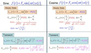
The following figure summarizes the transient and steady-state responses to both sine and cosine functions for directly excited SDOF system:

Time for Transient Response to Decay

Recall steady state and transient solution for sine harmonic excitation, the time that it takes for [latex]X_str< d X_o-ss[/latex] where d is the error percentage around the steady state solution can be found by: [latex]\frac{\Omega e^(\zeta \tau_d)}{\sqrt(1-\zeta^2)} -\frac{1}{\zeta} ln(\frac{d \sqrt(1-\zeta^2)}{\Omega})[/latex]. It should be noted that we know [latex]\tau_d=\omega_n t_d[/latex].

Undamped System: Resonance and Stability

For a system that is undamped (i.e. [latex]\zeta=0[/latex]), the equation of motion will be:

[latex]\ddot x(t)+\omega_n^2 x(t)=\frac{1}{m} F_0 sin(\omega t) u(t)[/latex]

1. Response when [latex]\omega\ne\omega_n[/latex], let [latex]\tau=\omega_n t[/latex].

Recall general solution: [latex]x(\tau)=[x_sss (\tau)+x_str (\tau)] u(\tau)[/latex].

After substituting [latex]\zeta=0[/latex], the solution will be simplified to:

[latex]x(t)=\frac{F_0}{k(1-\Omega^2)} [sin(\omega t)-\Omega sin(\omega_n t)][/latex]. If the excitation frequency is NOT equation to natural frequency for an undamped system, and if the ratio between excitation frequency and natural frequency is a rational number, the solution will be a perdioc solution. The solution will have a finite magnitude, therefore the solution is bounded and known as stable.

However, if the excitation frequency is equal to the natural frequency, the solution is not periodic, is unbounded, is unstable, and is known as a resonance relation.