OBJECTIVES

We shall show how to do the followings:

• Analyze single degree-of-freedom systems subjected to abruptly changing forces such as shocks, pulses, step functions, and ramps that are applied to the inertia element and to the base of the system.
• Relate the ratio of the duration of a time varying force to the period of free oscillation of the system.
• Determine the spectral content of the input disturbance and the response.
• Relate the characteristics of a transient to its frequency content and study how this affects the system response.

Introduction

Solution for Response to Transient Excitation

When the initial displacement [latex]X_0=0[/latex] and the initial velocity [latex]V_0=0[/latex], the solution for an underdamped system ([latex]0<\zeta<1[/latex]) is [latex]x(t)=\frac{1}{m\omega_d} \int_0^t \! e^{-\zeta \omega_n \eta} sin(\omega_d \eta)f(t-\eta) d\eta[/latex] where [latex]\eta[/latex] is the variable of integration and [latex]\omega_d=\omega_n \sqrt{(1-\zeta^2)}[/latex]

Response to Impulse Excication

Initially we need to define an impulse excitation mathematically. An impulse excitation is described by

[latex]f(t)=f_0 \delta(t)[/latex]

where [latex]f_0[/latex] is the magnitude of the impulse and has the units of [latex]N.s.[/latex] and [latex]\delta(t)[/latex] called the delta function, where

[latex]\int_{-\infty}^{\infty} \! \delta(t-t_0) g(t) dt= g(t_0)[/latex]

where [latex]g(t)[/latex] is assumed to be continuous at [latex]t=t_0[/latex]. Then,

[latex]x(t)=\frac{f_0}{m\omega_d} \int_0^t \! e^{-\zeta \omega_n \eta} sin(\omega_d \eta)f(t-\eta) d\eta[/latex] m

[latex]x(t)=\frac{f_0}{m\omega_d} e^{-\zeta \omega_n t} sin(\omega_d t)u(t)[/latex] m

Note: [latex]\deta (t)[/latex] has units equal to the reciprocal of its argument.

which in terms of the non-dimensional time [latex]\tau=\omega_n t[/latex] is

[latex]x(t)=\frac{f_0}{m\omega_n} \fract{e^{-\zeta \tau}}{\sqrt(1-\zeta^2)} sin(\sqrt(1-\zeta^2 \tau)u(\tau)[/latex]

when [latex]f_0=1[/latex], a unit impulse is said to be applied; that is

[latex]h(\tau)=\frac{1}{m \omega_n} \frac{e ^(\zeta \tau)}{\sqrt {1-\zeta^2}} sin (\sqrt{1-\zeta^2} \tau) u(\tau)[/latex]

where [latex]h(\tau)[/latex] is called the impulse response of the system.

Similarity to Response to Initial Velocity: 

The response for a system subjected to an initial displacement is given by:

[latex]x(\tau)=\frac{V_0}{\omega_n} \frac{e^{-\zeta \tau}}{\sqrt(1-\zeta^2)} sin(\sqrt{1-\zeta^2} \tau)[/latex]

Thus, one can see how we can assume the system will respond similarly and [latex]V_0=\frac{f_0}{m}[/latex]

Hence, the response of a system to an impulse can be determined as the response of a system with the corresponding initial velocity.

Extremum of Response to an Impulse:

The maximum displacement of the system subjected to an initial velocity [latex]V_0[/latex] can be used to obtain the maximum response to an impulse. Thus,

[latex]x_max=x(\tau_m)=\frac{V_0}{\omega_n}e^{-\phi/tan \phi}=\frac{f_0}{m \omega_n}e^{-\phi/tan \phi}[/latex]

[latex]\tau_m=\frac{\phi}{\sqrt{1-\zeta^2}}[/latex] and [latex]\phi=tan^-1 \frac{\sqrt{1-\zeta^2}{\zeta}}[/latex]

Foce Transmitted to the Boundary:

The force transmitted to the fixed boundary is

[latex]F_b=kx(t)+c \frac{dx(t)}{dt}=k[x(\tau_+2\zeta \frac{dx(\tau)}{d\tau}][/latex]

Figure 6-1 represents the normalized force versus different damping ratios. It is shown that around [latex]\zeta=0.25[/latex], the transmitted force to boundary is minimized to 81% of original value (i.e. undamped value).

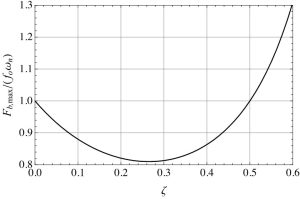
To obtain the maximum decrease in the amount of force transmitted to the base due to an impulse loading, the damping ratio should be between 0.2 and 0.35, which gives the maximum attenuation of the force transmitted of approximately 18%.

For a given damping ratio and given magnitude of the impulse force, decreasing the natural frequency decreases the magnitude of the force transmitted to the fixed boundary.

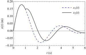
Example 6.1: Response of a linear vibratory system to multiple impacts

A system has a mass of 2 kg, a stiffness of 8 N/m, and a damping coefficient of 2 N s/m.  It is subjected to an impact of the form

[latex]f(t)=f_1(t)+f_2(t)=\delta (t)+ 0.5 \delta (t-1)[/latex]

The solution will be of the form

[latex]x(t)=x_1(t) u(t)+x_2(t-1) u(t-1)[/latex] Then, [latex]\omega_n=\sqrt{\frac{8 N/m}{2 kg}}= 2 rad/sec[/latex] and [latex]\zeta=0.25[/latex].

For the first impact, [latex]f_0=1 N.s.[/latex] and the response is given by:

[latex]x_1(t)=0.26 e^{-0.5t} sin(1.94t) u(t)[/latex]

For the second impact, [latex]f_0=0.5 N.s.[/latex] and the response is given by:

[latex]x_2(t)=0.13 e^{-0.5(t-1)} sin(1.94(t-1)) u(t-1)[/latex]

Thus, the total response is:

[latex]x(t)=0.26 e^{-0.5t} sin(1.94t) u(t)+0.13 e^{-0.5(t-1)} sin(1.94(t-1)) u(t-1)[/latex]

The total response of the system is shown below in Figure 6-2.

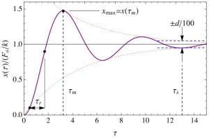
Response to Rectangular Pulse (Step) Input

The step input is given by: [latex]f(t)=F_0 u(t)[/latex]

After performing the convolution integral, the general form of the solution will be:

[latex]x(\tau)=\frac{F_0}{k}[1- \frac{e^{-\zeta \tau}}{\sqrt{1-\zeta^2}}sin(\tau \sqrt{1-\zeta^2}+\phi)]u(\tau)[/latex]

Some Terms: 

Three descriptors that are based on the response to a step input to characterize three important aspects of a linear system are:

Rise time – speed of response

Percentage overshoot – magnification of the response by the system

Settling time – speed at which the system can return to its equilibrium state.

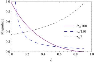
Rise Time: this is the time to go from 10% to 90% of the steady-state value.

Settling time: time it takes to be within +/-d% of the steady-state value.

Percentage overshoot: percentage difference between maximum value and steady-state value.

Design Limitations: 

For a linear single degree of freedom system with a mass m and a natural frequency [latex]\omega_n[/latex], the rise time, bandwidth, and percentage overshoot are a function of damping factor [latex]\zeta[/latex].

Selecting [latex]\zeta[/latex] to adjust any one characteristic affects the others.

Thus, for example, decreasing [latex]\zeta[/latex] (decreasing c) to decrease rise time increases the percentage overshoot and the settling time. This is shown in Figure 6-4.