Objectives:
- Compute the mass moment of inertia of rotational systems
- Compute the equivalent mass of complex systems
- Determine the stiffness of various elastic components in translation and rotational and the equivalent stiffness
- Determine the stiffness of fluid and pendulum elements
- Determine the potential energy of stiffness elements
- Determine the damping of systems that have different sources of dissipation
- Construct models of vibratory systems
Model Construction:
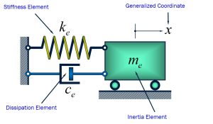
Our goal in any vibrational problem is to model a complex system and reduce it to a single mass, spring, and damper system. Each of these elements, shown in Figure 2-1, have different excitation-response characteristics that we will discuss further in this chapter.
The excitation is in the form of a force, or a moment and the corresponding response of the element is in the form of a displacement, velocity or acceleration.
Inertia Elements:
Inertia elements are characterized by a relationship between an applied force (or moment) and the corresponding acceleration response.
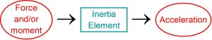
In other words, any force associated with an inertia element (i.e. mass element) can be found by using the Principle of Linear Momentum: [latex]F=ma[/latex] where F is the force, m is the mass and a is the acceleration.
Stiffness Elements:
Stiffness elements are characterized by a relationship between an applied force (or moment) and the corresponding displacement (or rotation) response.
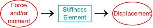
In other words, any force associated with a stiffness element (i.e. spring element) can be found by using the Hook’s Law: [latex]F=kx[/latex] where F is the force, k is the spring stiffness, and x is the displacement.
Dissipation Element:
Dissipation elements are characterized by a relationship between an applied force (or moment) and the corresponding translational or rotational velocity response.
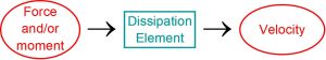
In other words, any force associated with a dissipation element (i.e. damping element) can be found by [latex]F=cv[/latex] where F is the force, c is the dissipation constant, and v is the velocity.
Translational and Rotational Motion:
The motions associated with different systems can be categorized to linear translational or rotational motions. The following table provides the equivalent terms for each of the motions:
| Quantity | Units |
| Translational motion
Mass, m Stiffness, k Damping, c External force, F
Rotational motion Mass moment of inertia, J Stiffness, kt Damping, ct External moment, M |
kg N/m N×s/m N
kg×m2 N×m/rad N×m×s/rad N×m |
Consider a mass m translation with a velocity of magnitude in the [latex]\dot x[/latex] plane [latex]X-Y[/latex].
Based on the Principle of Linear Momentum, the following mass (m) traveling with the velocity of [latex]\dot x[/latex] in the i-direction, will have a linear moment of [latex]p=m \dot r[/latex]. The force applied on it will be [latex]F=dp/dt[/latex]. Therefore, the force on the mass will be [latex]F=m \ddot x[/latex].
The kinetic energy of the mass will be the [latex]T=\frac {1}{2} m (\dot x i. \dot x i)= \frac{1}{2} m (\dot{x})^2[/latex].
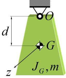
Rotational Motions of Mass: The inertia property is a function of the mass distribution as described by its mass moment of inertia about its center of mass or a fixed point O.
When the mass oscillates about a fixed point O or a pivot point O, the rotary inertia [latex]J_o[/latex] is given by the parallel-axes theorem:
[latex]J_o=J_G +md^2[/latex]
where m is the mass of the element, [latex]J_G[/latex] is the mass moment of inertia about the center of mass, [latex]d[/latex] is the distance from the center of gravity to the point O.
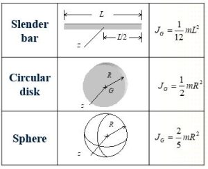
The following table provides a list of comment geometries and their mass moment of Interia about center of mass:
Example 2.1: Determine mass moment of inertia of the system below.
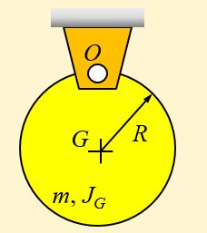
From the parallel axis theorem:
[latex]J_o=J_G+mR^2[/latex] where from Figure 2-6 we know [latex]J_G=\frac{1}{2}mR^2[/latex], therefore:
[latex]J_o=\frac{1}{2}mR^2+mR^2=\frac{3}{2}mR^2[/latex].
Example 2.2: Determine mass moment of inertia of the system below.
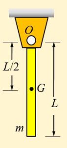
From Figure 2-6, we know [latex]J_G=\frac{1}{12}mL^2[/latex]. From the parallel-axis theorem we find:
[latex]J_o=J_G+m(L/2)^2=\frac{1}{12}mL^2+\frac{m}{4}L^2=\frac{1}{3}mL^2[/latex].
Example 2.3: Find the equivalent mass of the system shown below.
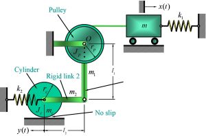
If we find the total kinetic energy of the system, we can then write [latex]T=\frac{1}{2}[m_eq][\dot x]^2[/latex]. Based on this expression, we can isolate the term [latex]m_eq[/latex].
We are assuming [latex]x(t)[/latex] is small. We are also considering [latex]x(t)[/latex] as the generalized coordinate system of the system and would like to write all other coordinates in terms of [latex]x(t)[/latex].
Therfore,
[latex]\theta(t)=x(t)/r_p[/latex] and[latex]y(t)=\theta(t)l_1=\frac{l_1}{r_p}x(t)[/latex].
We will then divide the system into individual components and find the kinetic energy of each separately.
Mass m is going through only translational motion. The kinetic energy of the mass [latex]m[/latex] can be found by:
[latex]T_1=\frac{1}{2}m\dotx^2[/latex]
The pulley p is going through rotational motion, it’s kinetic energy can be found by:
[latex]T_2=\frac{1}{2}J_p\dot\theta^2=\frac{1}{2}J_p(\dot\x/r_p)^2[/latex]
The vertical bar is also going through rotational motion since it is attached to the rotating pulley:
[latex]T_3=\frac{1}{2}J_1\dot\theta^2=\frac{1}{2}(m_1 (l_1)^2[/latex]
The horizontal bar is going through translational motion:
[latex]T_4=\frac{1}{2}m_2 \doty^2=\frac{1}{2}m_2 (l_1 \dotx/r_p)^2[/latex]
The rolling cylinder is going through both translational and rotational motion:
[latex]T_5=\frac{1}{2}m_c \dot y^2+\frac{1}{2}J_c \dot \phi^2[/latex] where [latex]\phi=y \times r_c=(l_1/r_p)x(t) r_c[/latex].
Therefore, [latex]T_5=\frac{1}{2}m_c (l_1 \dotx/r_p)^2+\frac{1}{2}J_c (l_1/r_p r_c)^2 (\dot x(t))^2[/latex]
At the end, we can add all the kinetic energies together:
[latex]T_total=T_1+T_2+T_3+T_4+T_5[/latex]
[latex]T_total=\frac{1}{2}m \dot (x)^2+\frac{1}{2}J_p \dot (x/r_p)^2+\frac{1}{2}(m_1 l_1^2/3) \dot (x)^2 /(r_p)^2+\frac{1}{2}m_2 (l_1/r_p \dotx)^2+\frac{1}{2}(l_1/r_p \dot x)^2[/latex]
The equivalent mass can be found by reorganizing the above kinetic term and writing this in this form: [latex]T_total=\frac{1}{2} m_eq \dot(x)^2[/latex].
Stiffness Element and Their Combinations:
[latex]F_s[/latex] is the internal force acting within the stiffness element. It is called the restoring force. As the stiffness element is deformed, energy is stored in this element, and as the stiffness element is un-deformed energy is released. This energy is called potential energy.
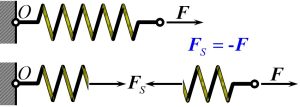
The potential energy V is defined as the work done to take the stiffness element from the deformed position to the un-deformed position; that is, the work needed to un-deform the element to its original shape.
Springs can be in series or parallel. When springs are in series, the springs have the same force. When the springs are in parallel, the springs have the same displacement. Equivalent spring constant for springs in series is:
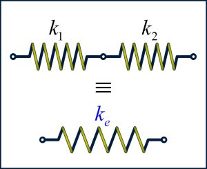
The equivalent spring constant is [latex]k_e=\frac{k_1 k_2}{k_1+k_2}[/latex].
Equivalent spring constant for springs in parallel is:
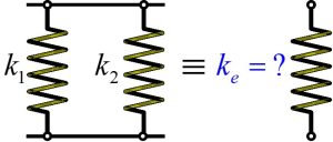
The equivalent spring constant is [latex]k_e=k_1+k_2[/latex].
Structures Modeled as Springs
A few equivalent springs constants of common structural elements used in vibratory models are listed below:
- Axially Loaded Rod or Cable
-
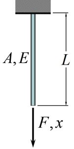
Figure 2-13: Axially Loaded Rod [latex]k=\frac{AE}{L}[/latex]
-
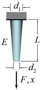
Figure 2-14: Changing Cross Section Area of Axially Loaded Rod [latex]k=\pi E d_1 d_2 /4L[/latex]
Cantilever Beam:
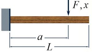
[latex]k=3EI/a^3[/latex]
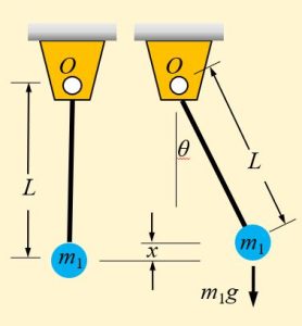
Pendulum Systems:
Pendulum System Example 1: Find the equivalent spring constant of the pendulum system shown below by using the potential energy equation.
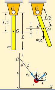
Recall that for a pendulum: [latex]y=h-Lcos\theta[/latex]. In the present notation,
[latex]y is x and h is L/2 and L is L/2.[/latex] and we obtain [latex]x=L/2 - L/2 cos \theta =\frac{L}{2} (1-cos \theta)[/latex]. Since [latex]F=-mg j[/latex], the increase in the potential energy is: [latex]V(x)=mgx[/latex].
This can be written as [latex]V(\theta)=mgL/2 (1-cos \theta)[/latex].
From the Taylor series approximation for [latex]cos \theta= 1- \theta^2/2+...[/latex], we obtain
[latex]V(\theta)=mgL/2 (1-cos \theta)=mgL2 (1-[1-\theta^2/2])[/latex]
therefore, [latex]V(\theta)=(1/2)k_te \theta^2[/latex] where [latex]k_te=mgL/2[/latex].
Pendulum System Example 2: Find the equivalent spring constant of the pendulum system shown below by using the potential energy equation.
Using the previous results by replacing L/2 with L: [latex]x=L(1-cos \theta)[/latex]
The potential energy is [latex]V(\theta)=(1/2)k_te \theta^2[/latex]
where we replace [latex]m[/latex] with [latex]m_1[/latex] and [latex]L/2[/latex] with [latex]L[/latex] to obtain [latex]k_te=m_1 g L[/latex].
Dissipation Elements and Their Combinations:
Damping elements are assumed to have neither inertia nor the mean to store or release potential energy.
The mechanical motion imparted to these elements is converted to hear or sound and, hence, they are called non-conservative or dissipative because this energy is not recoverable by the mechanical system. The following are four common types of damping mechanisms:
- Viscous damping
- Coulomb or dry friction damping
- Material or solid or hysteretic damping
- Fluid damping
In these cases, the damping force is usually expressed as a function of velocity.
Viscous Damping: When a viscous fluid flows through a slot or around a piston in a cylinder, the damping force generated is proportional to the relative velocity between the two boundaries confining the fluid.
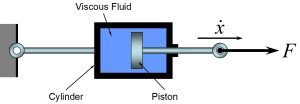
The equation associated with the viscous damping can be written as:
[latex]F(\dot x)=c \dot x[/latex]
where [latex]c[/latex] is the Damping Coefficient and has the units of [latex]N/(m/s)[/latex]. The energy dissipated by a linear viscous damper is given by:
[latex]\int_{}^{} F \,dx=\int_{}^{} F \dot x \,dx=\int_{}^{} c (\dot x)^2 \,dx=c \int_{}^{} (\dot x)^2 \,dx[/latex].\
Linear viscous damping elements can be combined in the same way that linear springs are, except that the forces are proportional to velocity instead of displacement.
When dampers are in series, the force on each damper is the same.
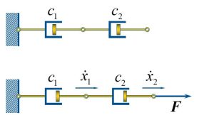
If we write the force on the first damper, it will be: [latex]F=c_1 \dot x_1[/latex] whereas the force on the second damper will be [latex]F=c_2 (\dot x_2- \dot x_1)[/latex]. In each equation, we solve for:
[latex]\dot x_1=F/c_1[/latex]
and [latex]\dot x_2 -\dot x_1=F/ c_2[/latex]. Lets substitute [latex]\dot x_1=F/c_1[/latex] into the second equation and we get:
[latex]\dot x_2=F/c_1 + F/c_2 =F (1/c_1 + 1/c_2)[/latex]. Now, the equation can be simplified to:
[latex]F=(1/c_1 + 1/c_2)^-1 \dot x_2[/latex] then [latex]c_e=\frac{c_1 c_2}{c_1+c_2}[/latex].
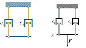
If dampers are in parallel, the velocities are the equal. Therefore, we can write the equivalent damping coefficient to be [latex]c_e=c_1+c_2[/latex].
Model Construction:
Discrete system or a lumped-parameter system: Only discrete elements are used to model a physical system: mass, stiffness and damping. These three types of elements appear as parameters in the governing equations of the system.
Distributed-parameter system or continuous system: No discrete elements are used to model the system. One or more partial differential equations are used to model the system. Equivalent to an infinite number of discrete elements.