7
Dr. Kevin Bracker; Dr. Fang Lin; and jpursley
Learning Objectives
After completing this chapter, students should be able to
- Define the concept of risk and explain how both the probability and magnitude of outcomes impact the degree of risk.
- Identify sources of risk and differentiate between general economic risk factors and firm specific risk factors.
- Explain the concepts of probability distributions, expected return and standard deviation for a single security.
- Calculate and interpret the expected return and standard deviation of a single security given a probability distribution.
- Explain the concept of correlation.
- Explain the concept of expected return and standard deviation for portfolios.
- Calculate and interpret the expected return and standard deviation for two-stock portfolios.
- Explain/diagram the concept and implications of portfolio diversification.
- Differentiate between firm-specific (diversifiable) risk, market (non-diversifiable) risk, and total risk.
- Identify when each risk type of risk measurement is appropriate.
- Calculate and interpret beta.
- Explain, calculate, and interpret the Capital Asset Pricing Model and Security Market Line.
- Identify potential concerns regarding the viability of the Capital Asset Pricing Model and the Security Market Line
What is Risk?
Risk refers to the possibility of an unfavorable event occurring. The higher the risk, the greater the probability of an unfavorable event or the more unfavorable the event could be. The interaction of the probability of the unfavorable event and the degree of negativity associated with the event is critical to determining the risk.  For instance, imagine that you are going to participate in a coin flip. It will cost you $1.00 to participate. If you flip a head, you get $1.01. If you flip a tail you get $0.99. Even though there is a fairly high probability of the unfavorable event (50% chance of tails), the outcome is so minor (you lose $0.01) that this would be a low-risk event. Now, consider a slightly different coin flip. This time, instead of flipping the coin once, you will flip it 3 times. If you get 3 heads, you receive $10,000. If you flip 3 tails, you owe $10,000. Anything else you get your $1.00 back. Even though the probability of the bad outcome is much smaller (there is only a 12.5% chance of flipping 3 straight tails), this is a much riskier event due to the bad outcome being substantially worse. However, most people do not consider flying a commercial airliner to be a high risk event (even though the worst case scenario is obviously quite severe) because of the extremely low probability of a fatal crash (less than 1 in 10 million). It is not just the probability or just the degree of unfavorable outcome, but the combination of the two that matter for rational risk analysis.
In finance terms, our “unfavorable event” refers to earning less than expected. Any time we have a chance to earn less than expected on an investment opportunity we are exposed to risk. Note that this is a more strict definition than defining risk as the possibility of losing money. We want to be careful to think of risk as the possibility of earning less than expected instead of being the possibility of losing money.
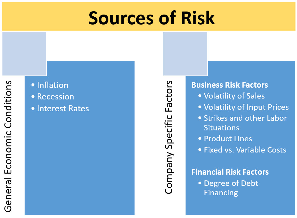
Note that the above list is a sample of broad factors and not a specific list. For example, consider what happens when we have a large increase in oil and gasoline prices. One immediate impact is inflation. The higher energy prices are, by definition, inflation in energy, but it goes beyond that. Now it costs more for firms to distribute their products to suppliers which is likely to cause the inflation to spill over to other areas. As we search for alternative energy sources (like ethanol), we may see corn prices rising. Since corn is used to feed cattle, this could lead to an increase in beef costs as well. Also, if consumers are now spending more to fill up their gas tanks and more to buy a variety of food products, there would be less money available to spend on entertainment and other goods/services. This could lead to a recessionary environment (could, not will, because there are always so many influences on the economy that this is just one of many factors impacting economic growth). The point here is not the specific impacts of higher oil/gasoline prices, but that many economic risk factors may have more complex interactions than are apparent at the surface.
One other thought on risk to keep in mind as we move through this chapter. Throughout the chapter, we will be treating risk and potential returns as largely objective and measurable. However, in practice, one of the biggest challenges of risk management is trying to figure out what bad outcomes are and how likely they are. As, John Kenneth Galbraith, one of the great economists of the 20th century once wrote – “There are two kinds of forecasters: those who don’t know, and those who don’t know they don’t know.” In practice, the results of our models are only as good as the inputs we put into them.
Diversification
Diversification refers to the concept that by holding a number of different securities (ideally not just stocks) from a spectrum of industries, we can negate the impact of company specific factors on our returns. We will come back to this issue (one of the most important concepts in finance) in more detail later in this chapter.
Expected Return and Standard Deviation of a Single Security
Expected Return
The expected return of a security is based on the probability distribution of returns. Before we get into the details of the expected return, let’s briefly introduce the concept of a probability distribution. A probability distribution is a representation of possible outcomes (states of nature) that may occur and the likelihood (probability) of each outcome. If you think of a coin flip, the probability distribution has two possible outcomes (heads or tails) and each outcome has a 50% chance of occurring (technically, this is not true as even in a “fair” coin flip, the side that starts up has about a 51% chance of occurring). When dealing with financial securities, the number of possible outcomes is nearly infinite and it is not possible to know the exact outcomes or probabilities of those outcomes. Therefore, we are really only approximating the true probability distribution.
Video Probability Distribution
Specifically, the expected return is the probability of a specific state of nature occurring times the return under that state of nature summed across all possible states of nature. In formula terms, it is
[latex]\bar{k}=\sum_{i=1}^{n} P_{i}k_{i}[/latex]
OR
[latex]\bar{k}=P_{1}k_{1}+P_{2}k_{2}+...+P_{n}k_{n}[/latex]
where
[latex]\bar{k}[/latex] represents the expected return of the stock
Pi represents the probability of the ith possible outcome (state of nature)
ki represents the return under the ith outcome (state of nature)
Pn represents the probability of the nth possible outcome (state of nature)
kn represents the return under the nth outcome (state of nature)
Don’t worry if the formula and definition seem intimidating, the process is relatively simple. Consider the following example. After researching Stock A we have determined that there are 3 possible outcomes for the next year (3 states of nature). The first possibility is the economy enters a recession causing the stock to have a return of -15%. The probability of this occurring is 20%. The second possibility is that the economy goes smoothly, but does not experience rapid growth causing the stock to rise and offer a 10% return. The probability of this occurring is 50%. The third possibility is that the economy booms, causing the stock to provide a 35% rate of return. The probability of the economy booming is 30% (note that the probabilities must sum to 1.0 and the states of nature should be mutually exclusive).
| State of Nature | Probability | Return |
| Recession | 0.20 | -15% |
| Normal | 0.50 | 10% |
| Boom | 0.30 | 35% |
What is the expected rate of return?
[latex]\bar{k}=(.20)(-15\%)+(.50)(10\%)+(.30)(35\%)[/latex]
[latex]\bar{k}=-3\%+5\%+10.5\%[/latex]
[latex]\bar{k}=12.5\%[/latex]
Video Expected Return of a Single Security
Standard Deviation
The standard deviation measures the variability of possible returns and is represented by the lower-case Greek symbol sigma. The smaller the standard deviation, the more likely we are going to earn something “close” to our expected return. The greater the standard deviation, the greater the chance that we may earn something far more (good) or far less (bad) than our expected return. The formula for this is (remember that [latex]\bar{k}[/latex]is our symbol for expected return):
[latex]\sigma=\sqrt{\sum_{i=1}^{n}P_{i}(k_{i}-\overline{k})^2}[/latex]
OR
[latex]\sigma=\sqrt{P_{1}(k_{1}-\overline{k})^2+P_{2}(k_{2}-\overline{k})^2+...+P_{n}(k_{n}-\overline{k})^2}[/latex]
where
sigma (σ) represents the standard deviation
Pi represents the probability of the ith outcome (state of nature)
ki represents the return under the ith outcome (state of nature)
[latex]\bar{k}[/latex] represent the expected return for the stock
Pn represents the probability of the nth outcome (state of nature)
kn represents the return under the nth outcome (state of nature)
Calculation Notes:
It is easy to get confused with decimals and percents. The best way to do these calculations is to always leave the weights as decimals and the returns as a regular number. For instance, if you have a probability of 0.10 and a return of 15%, you would put the probability into your calculator as 0.10 and the return as 15.
Be careful with your order of operations.
- Do (k1 – [latex]\bar{k}[/latex]) first
- Then square that
- Then multiply by P1
- Repeat for all n states of nature
- Add them up
- Finally, take the square root
Consider our previous example. What is the standard deviation for stock A?
[latex]\sigma=\sqrt{0.2(-15-12.5)^2+0.5(10-12.5)^2+0.3(35-12.5)^2}[/latex]
[latex]\sigma=\sqrt{0.2(756.25)+0.5(6.25)+0.3(506.25)}[/latex]
[latex]\sigma=\sqrt{151.25+3.13+151.88}[/latex]
[latex]\sigma=\sqrt{306.25}[/latex]
[latex]\sigma=17.50\%[/latex]
Video Standard Deviation of a Single Security
Interpreting Expected Return and Standard Deviation
Expected return gives us an idea of how much we will make on the investment. Remember that it is not how much we will make, but how much we would make on average if we could repeat the holding period an infinite number of times. Think of a situation where you are asked to pick a number between 1 and 10. If you select the correct number you get $100 and if not you get nothing. Any one time that you try this, you will either receive $100 (if you are lucky) or $0. However, if you could repeat the exercise 100,000 times, you would find that you would make almost exactly $10 per time. It is critical to know expected values when selecting investments. For instance, if someone offered you the opportunity to do this exercise for $9 per pick and you could pick as often as you wanted, it would be an excellent opportunity. Alternatively, if you were offered the same thing for $11, you would (hopefully) walk away. However, it is just as important to understand that the expected return is only an average return and not the return you will receive in any particular instance. This example also illustrates why it is so important to focus on the process and not the result. If you had the opportunity to play this game once for a cost of $2 and you lost, it still was a smart decision to play and you should do it again if you got the chance. If you had the opportunity to play this game once for a cost of $20 and you won, it was still a bad decision to play and you should pass if offered the opportunity to try again.
Now consider a similar exercise — pick a number between 1 and 5. If you select the correct number, you get $50 and if not you get nothing. The expected value for this exercise is the same as the previous exercise ($10). So, imagine that you are offered the opportunity to participate in either one (pick from 10 numbers or pick from 5 numbers) for $8. You can only play once. Most people will now choose to pick from 5 numbers. Why? Because it has less risk (a lower standard deviation) and offers the same expected return. This is the concept of risk aversion. As a side note, if you still picked the 10-number game it is likely because the stakes are small (the entertainment value of the gamble outweighs the financial aspect). As the stakes increase, the vast majority of people will choose the 5-number game.
Moving away from our example, let’s put this in finance terms. Consider two stocks. Stock A has an expected return of 10% and a standard deviation of 25%. Stock B has an expected return of 10% and a standard deviation of 30%. Which should you choose and why? (Answer to follow …think about it first)
Now consider two other stocks. Stock C has an expected return of 7% and a standard deviation of 20%. Stock D has an expected return of 9% and a standard deviation of 28%. Which should you choose and why? (Again, spend some time thinking before reading the next paragraph).
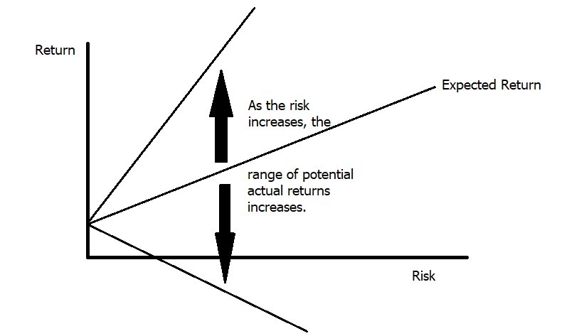
In the first example, you should choose stock A and so should everyone else. Stock B offers us no additional compensation (expected return) to entice us to take the higher risk (standard deviation). Therefore, it is irrational in a risk-averse framework to invest in stock B. In the second example, you could choose stock C or stock D and someone else may make the same choice or the opposite choice. Here, the choice is based on your individual level of risk aversion. Stock D is riskier, but it also compensates us for that risk with a higher expected return. Is the compensation enough? That depends on the individual. For those that are less risk-averse, they require less additional compensation to take on the extra risk so they will likely take stock D. For those that are more risk averse, they will take stock C because the extra compensation is not enough for them to take the extra risk. Take a few moments and try to think of what factors impact your level of risk aversion. Typically we find that age, personality, number of dependents, wealth, income, variability of income, past life experiences, and other factors all combine to influence one’s level of risk aversion. One last thought — remember that taking stock D does not mean you will earn a higher return, just that you will earn a higher return on average. If you always earned a higher return from stock D, then it wouldn’t be riskier. Visually, you can think of it along the lines of the diagram below. At low levels of risk the range of returns will be close to the expected return. At high levels of risk, the range of returns will be higher. The expected return increases with risk, but so to does the range of potential returns.
Graph: Range of Potential Actual Returns
Expected Return and Standard Deviation of a Portfolio
Expected Return
The expected return for a portfolio is simply the weighted average of each stock held in the portfolio. The formula here is
[latex]\bar{k_{p}}=\sum_{i=1}^{n}W_{i}\bar{k_{i}}[/latex]
OR
[latex]\bar{k_{p}}=W_{1}\bar{k_{1}}+W_{2}\bar{k_{2}}+...+W_{n}\bar{k_{n}}[/latex]
where
[latex]\bar{k_{p}}[/latex] represents the expected return for the portfolio
W1 represents the weight (proportion of portfolio) of stock 1
[latex]\bar{k_{1}}[/latex] represents the expected return for stock 1
Wn represents the weight (proportion of portfolio) of stock n
[latex]\bar{k_{n}}[/latex] represents the expected return for stock n
Again, let’s consider an example. What is the expected return of a portfolio made up of 60% Stock A and 40% Stock B when the expected return for Stock A is 10% and the expected return for Stock B is 20%?
[latex]\bar{k_{p}}=(.60)(10\%)+(.40)(20\%)[/latex]
[latex]\bar{k_{p}}=6\%+8\%[/latex]
[latex]\bar{k_{p}}=14\%[/latex]
Video Expected Return of a Two-Stock Portfolio
Standard Deviation
The standard deviation of a portfolio becomes more complicated. It depends not only on the standard deviation and weightings of each stock, but also on the correlation between pairs of stocks.
Correlation
The correlation between a pair of stocks measures how closely the returns for each stock are related. A negative correlation means that the price of one stock tends to fall while the other rises (prices/returns are inversely related). A positive correlation means that the price of one stock tends to rise while the other rises (prices/returns are positively related). Correlations can range from -1.0 to 1.0. Correlations for real-world variables are almost never at the extremes (perfect positive correlation, no correlation, or perfect negative correlation).
See the Observed Betas, Correlations, and Standard Deviations Table in Appendix B for some standard deviations and correlations from actual companies over the past five years.
Observations from the Table
- The last two rows/columns are for an aggregate US bond fund and the S&P 500 ETF. The purpose of these is to provide a proxy for the US bond market and the US stock market.
- The vast majority (65 of 66) of correlations between pairs of stocks are positive. This is because all stocks are impacted by general economic factors.
- The average correlation across pairs is a low, positive value (0.31 in our sample). While general economic factors cause a tendency for stock to move together, firm-specific factors push correlations towards zero.
- Stocks in similar industries tend to have higher correlations than the average stock (0.50 vs. 0.31).
- Each stock has a positive correlation with the overall stock market.
- The stock and bond market have a negative (although essentially zero) correlation during this time-period.
- The bond market has a much lower standard deviation than the stock market, but also generated much lower returns during this time-period.
- Most individual stocks have a standard deviation that is higher than the overall stock market. This is because the stock market represents a diversified portfolio which has eliminated most of the firm-specific risk. The exception is Pepsi in our sample which is essentially the same standard deviation.
- The historical annualized returns are not the same as the expected returns. It is unrealistic to expect 30%+ annual returns for Deere, Boston Beer or Amazon going forward (which is not the same as saying that these stocks can’t generate those returns). Also, it is unreasonable to expect people to buy stock in Molson Coors and Exxon with the anticipation of losing nearly 12% or 8% each year.
- While standard deviations will vary depending on overall market conditions, large cap stocks over this 5-year window had standard deviations of approximately 15-42%. Note that the standard deviations will be bigger or smaller depending on both the stock and the time period and that Boston Beer’s 42.5% is noticeably larger than the next closest company.
Standard Deviation for a two-stock Portfolio
In order to calculate the standard deviation of a two-stock portfolio, we will use the following formula:
[latex]\sigma_{p}=\sqrt{W_{1}^2\sigma_{1}^2+W_{2}^2\sigma_{2}^2+2W_{1}W_{2}\sigma_{1}\sigma_{2}corr_{1,2}}[/latex]
where
σp represents the standard deviation of the portfolio
W1 represents the weight (proportion of portfolio) of stock 1
σ1 represent the standard deviation of stock 1
W2 represents the weight (proportion of portfolio) of stock 2
σ2 represent the standard deviation of stock 2
corr1,2 represents the correlation between the returns of stocks 1 and 2
Again, let’s work through an example. Consider a two-stock portfolio in which 60% of your money is invested in stock A and 40% of your money is invested in stock B. Stock A has a standard deviation of 50% and stock B has a standard deviation of 70%. The correlation between the returns for stock A and stock B are 0.30. You want to find the standard deviation of this portfolio.
[latex]\sigma_{p}=\sqrt{(0.6)^2(50)^2+(0.4)^2(70)^2+2(0.6)(0.4)(50)(70)(0.3)}[/latex]
[latex]\sigma_{p}=\sqrt{(0.36)(2500)+(0.16)(4900)+(504)}[/latex]
[latex]\sigma_{p}=\sqrt{900+784+504}[/latex]
[latex]\sigma_{p}=\sqrt{2188}[/latex]
[latex]\sigma_{p}=46.78\%[/latex]
Note that in this example, the standard deviation of the portfolio is less than the standard deviation of either stock separately. This illustrates the concept of diversification. As long as the correlation is less than 1.0 (which it will be for any two stocks), the risk of the portfolio is less than the weighted average risk of the two securities which make up the portfolio (and sometimes — like here — even less than the lowest risk stock in the portfolio). While we will not cover the process of calculating the expected return and standard deviation for larger portfolios in this class, in practice, most portfolios hold far more securities.
Video Standard Deviation of a Two-Stock Portfolio
Diversifiable and Non-Diversifiable Risk
Remember earlier we discussed the possibility of lowering our firm-specific risk by holding a number of stocks from a wide range of industries? This concept of diversification allows us to greatly reduce our risk by holding a portfolio. Diversifiable risk refers to risk factors that are isolated towards one particular firm or industry.
For example, if a drug manufacturer gets hit with a lawsuit related to one of the drugs it produces, that is likely to have an isolated impact. It will not have any effect on the stock prices of auto manufacturers, grocery retailers, banks, etc. Once we have enough stocks in our portfolio, bad news for any one of them will have a small impact on our overall portfolio as long as that bad news is contained to that one firm (in other words, as long as it comes from a diversifiable risk factor). By holding approximately 25-50 stocks, we can eliminate a large portion of our diversifiable risk. (Statman, 1987) While a portfolio of 10 stocks has much less risk than a portfolio of 5 stocks, a portfolio of 100 stocks offers very little risk reduction compared to a much smaller 50-stock portfolio (assuming our stocks are from a variety of different industries and have other differing characteristics).

Does this mean that we have eliminated all of our risk when we hold a 50-stock (or even 500-stock) portfolio? No, we are still subject to general economic risk that affects all securities. This leftover risk is referred to as Non-diversifiable risk (or market/systematic risk). Examples of non-diversifiable risks include political events (such as wars), energy price shocks, changes in interest rates, recessions, etc. Any risk factor that impacts virtually all stocks is referred to as a non-diversifiable risk factor because it will impact our portfolio regardless of how well we have diversified our investments. Another name for non-diversifiable risk is “market risk” because these sources of risk tend to affect the entire market as opposed to an individual security or industry. Note: Market risk does not refer to risk impacting a specific industry. Instead it refers to risk impacting the broad economy (most stocks). If a risk factor only impacts one or two industries without carrying over to the broader market it is classified as firm-specific.
The following graph does a good job of illustrating the concept of diversification and firm-specific vs. market risk.
Graph: Firm-specific Risk vs. Market Risk
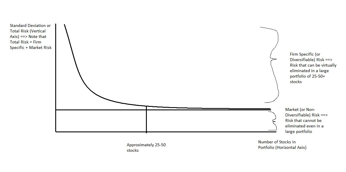
Given the relative ease with which investors can virtually eliminate their firm-specific (diversifiable) risk, for most investors the level of non-diversifiable (market) risk associated with an investment becomes more important. It is important to note that while market risk impacts all stocks, it does not impact all stocks equally. Therefore, we need to a tool to measure how sensitive a stock is to the overall market. This tool is known as BETA. Standard deviation measures total risk (diversifiable risk + market risk) for a security, while beta measures the degree of market (non-diversifiable) risk. We won’t introduce a risk measurement for diversifiable risk.
Video Diversification
Beta
In addition to serving as a measure of market risk, Beta tells us how a particular stock moves in relation to the rest of the stock market as a whole.
[latex]\beta_{A}=\frac{(\sigma_{A})(corr_{A,MKT})}{\sigma_{MKT}}[/latex]
where
βA represents the Beta of Stock A
σA represents the standard deviation of stock A
corrA,MKT represents the correlation between stock A and the overall market
σMKT represents the standard deviation of the overall market
Consider the following example. Stock A has a standard deviation of 60% while the overall stock market has a standard deviation of 25%. Assuming that the correlation between Stock A and the overall market is 0.30, what is the beta of Stock A?
Beta = [(60)(.30)]/(25) = 18/25 = .72
What is the Market?
The market refers to a portfolio of all investment assets (stocks, bonds, gold , art, etc.). However, in more practical terms, the market usually refers to the stock market and can be measured by a market index (such as the S&P 500 or Dow Jones Industrial Average).
How do we Interpret Beta?
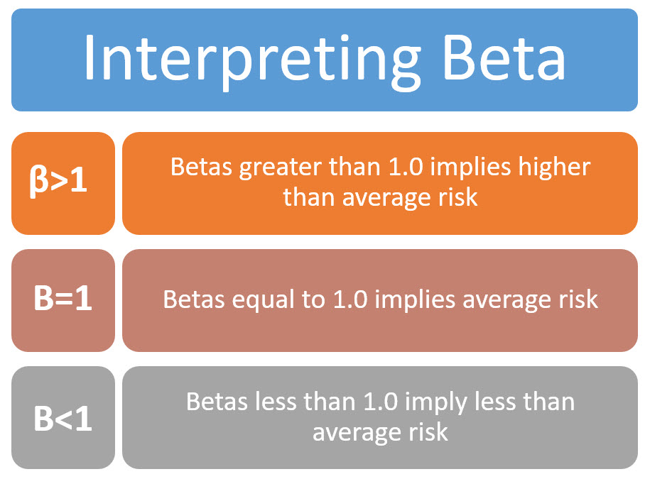
Most betas range between 0.35 and 1.8 (there are many outside this range, but the majority of stocks fall in this range – review Observed Correlations, Returns, Standard Deviations and Betas Table in Appendix B and note that all the stocks other than Wal-Mart fall in this window.)
Go back to our example where we calculated the beta for stock A. By itself, stock A is much riskier than the overall market as determined by its standard deviation. However, when we consider it as part of an overall portfolio its risk is much lower (less than average) due to the fact that it has a relatively low correlation to the overall market. The riskiness of stock A depends on whether we plan to use it as a stand alone investment or as part of a portfolio.
Standard Deviation vs. Beta
At this point, we have introduced two risk measurements. The first is standard deviation and the second is beta. In some cases, these two risk measurements will tell a different story. For instance, stock A may have a standard deviation of 30% and a beta of 0.8 while stock B may have a standard deviation of 25% and a beta of 1.3. Which stock is riskier? The answer is depends on the specific situation. Because each risk measurement is measuring a different type of risk (standard deviation measures total risk while beta measures market risk), we need to think of situations where each is appropriate.
Single Security and/or Poorly Diversified Portfolio
If you are going to place your entire investment into a single security or a poorly diversified portfolio, then standard deviation is the appropriate risk measurement. In this situation, you have not diversified away the majority of the firm-specific risk, so you need to include it in your analysis. Standard deviation does this because it includes both sources (market and firm-specific) of risk.
Adding a Security to a Well-Diversified Portfolio
If you own a well-diversified portfolio and you are planning to add a single security to that portfolio, then the firm-specific risk of the security you are adding is not relevant. The reason it is not relevant is because it will be one of many stocks in the large portfolio and the firm-specific risk will be diversified away. What matters is how that stock moves with the overall market. Since we measure this market risk with beta, our appropriate risk measurement here is beta.
Choosing Between 2 (or more) Well-Diversified Portfolios
If you are choosing between two or more portfolios that are each well-diversified, then you can use either standard deviation or beta as your risk measurement. The reason for this is that at this point, the firm-specific risk is already diversified away so that your total risk and market risk should be essentially the same. Thus, whichever portfolio has the higher standard deviation should also have the higher beta (if not, you know the portfolios are not well-diversified).
Beta and Required Return: Capital Asset Pricing Model (CAPM)
During the mid-1960’s and early-1970’s some finance professors developed the Capital Asset Pricing Model (CAPM). (Sharpe, 1964; Lintner, 1965; Black, 1972) One of the key components of this model is the Security Market Line (SML) which states that the required rate of return for a stock is dependent on the beta of that stock. While technically, the SML is a subset of the larger model (CAPM), in practice the two terms are typically used interchangeably. Thus, think of them as the same basic model. Specifically, the SML states that
[latex]k_{A}=k_{RF}+\beta_{A}(\bar{k_{m}}-k_{RF})[/latex]
where
kA is the required return for stock A,
kRF is the risk-free rate of interest (often approximated by the yield on 10-year Treasury bond),
βA is the beta for stock A,
[latex]\bar{k_{m}}[/latex] is the expected return on the market (often approximated by the S&P 500)
Let’s calculate the required return for a particular stock. Stock B has a beta of 1.4. The expected return on the market is 11% and the Treasury bond rate is 5%. Based on this, we can calculate the required return for stock B as follows
k = 5% + (1.4)(11% – 5%)
k = 5% + (1.4)(6%)
k = 5% + 8.4%
k= 13.4%
Video Beta and the SML Part One
Video Beta and the SML Part Two
Important Implications of the CAPM/SML
- According to the SML, high beta stocks should, on average, earn higher returns than low beta stocks.
- According to the SML, the only factor that should cause consistent differences in returns across stocks is beta.
- When interest rates rise, required returns should increase and (all else equal) cause stock prices to decline.
- When investors become more risk-averse, the risk premium [latex](\bar{k_{m}}-k_{RF})[/latex] should increase which will increase required returns and (all else equal) cause stock prices to decline.
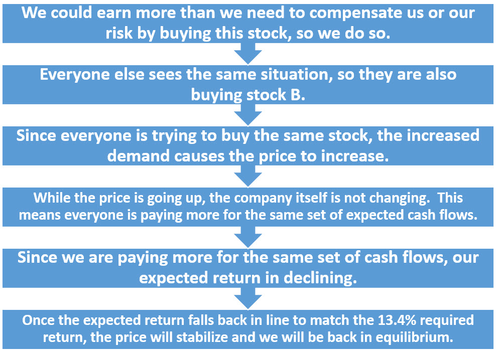
Under equilibrium conditions, the required return should equal the expected return. Let’s consider this for a minute. In our example above, we estimated that the required return for stock B should be 13.4%. What would happen if the expected return [latex]\bar{k}[/latex] for this stock was 16%?
For practice in understanding this concept, think through what would happen if the required return was 13.4% and the expected return was 9%. Also, think about what types of things may push us out of equilibrium and why this is relevant for explaining stock price movements.
Empirical Findings of the SML
While the CAPM/SML met with a lot of early success and became the standard for estimating required returns in the field of finance very quickly, it ran into problems in the 1990’s and is deemed less reliable at the moment. (Fama and French, 1992) There have been some alternative models (Fama-French 3-Factor model, Carhart 4-Factor model, Fama-French 5-Factor model, and the q-Factor model) introduced since then, however there has not been a new standard-bearer to take its place. As of right now, the SML is still commonly used in practice, however there is growing focus on the alternatives. My view is that it is critical for you to know and understand the basic premise of the CAPM and SML (that role of market risk in explaining returns) but also to be aware of some of the problems (listed below).
- While market returns play a major role in explaining returns of individual stocks, Beta doesn’t do a very good job of explaining future returns. In other words, after controlling for other factors, it is not clear that high beta stocks actually outperform.
- Small firms seem to earn higher returns than can be explained by beta.
- Firms with a low market-to-book ratio (MV/BV) tend to earn higher returns than can be explained by beta.
- Firms that have been top performers in the past 6-12 months tend to earn higher returns in the following 6-12 months than can be explained by beta.
Again, the above flaws do not mean that the CAPM/SML are useless. They provide a simplified framework for understanding how market risk relates to returns. However, recognize that they are not perfect models and the process of understanding stock returns is more complex than the SML indicates. As our knowledge increases, better models will likely evolve.
Key Takeaways
The relationship between risk and return is an essential element of financial analysis. Because investors tend to behave in a risk-averse manner, we anticipate that higher risk investments should have higher expected returns. In this chapter, we formalize that analysis by introducing measures of risk (standard deviation and beta) and expected return. Standard deviation captures the dispersion of possible returns (total risk) and is best used when evaluating individual investments in isolation or poorly diversified portfolios. Beta captures the risk of securities relative to the overall market (market risk) and is best used when evaluating individual investments within a portfolio. A portfolio represents a collection of securities held together and is an essential tool for diversifying away firm-specific risk. The lower the correlation between a pair of securities, the more potential diversification benefits there are. This is reminiscent of the “don’t put all your eggs in one basket” cliché. While diversification can virtually eliminate the impact of firm-specific risk, it cannot eliminate market risk. Therefore, investors should be compensated for the degree of market risk that they are exposed to in their investments. The Security Market Line (SML) formalizes the risk-return tradeoff with respect to beta, the risk-free rate, and the market risk premium. It hypothesizes that higher beta stocks should generate higher returns and beta should be the only factor that systematically differentiates returns. Unfortunately, the SML has not held up well to empirical testing which has led to the introduction of newer attempts to formalize the relationship between risk and return. While the specific nature of risk and return is not finalized, it is safe to say that, in general, higher risk should be rewarded with higher expected returns. However, it is important to remember that expected returns are not the same as realized returns due to the nature of risk.
Exercises
Question 1
What is Risk? What two factors are important in determining the degree of risk?
Question 2
“As long as we can’t lose any money, we have a risk-free investment.” Discuss this comment.
Question 3
Both investing and gambling can be defined as “undertaking risk in order to earn a profit.” Explain how these two activities are different and why society generally takes a more favorable view of investing compared to gambling.
Question 4
Explain the concept of correlation? If two securities have a high positive correlation what does that mean? Give an example of two securities that might be highly correlated. If two securities have a low positive correlation what does that mean? Give an example of two securities that might have a low positive correlation. If two securities are negatively correlated what does that mean? Give an example of two securities that might be negatively correlated?
Question 5
What is diversifiable risk? What is market or non-diversifiable risk? Give an example of each.
Question 6
Standard deviation measures what kind of risk? When is this important? When is it not important?
Question 7
Beta measures what kind of risk? When is this important? When is it not important?
Question 8
Explain why we can use either beta or standard deviation when comparing two well-diversified portfolios. Is this true for any two portfolios?
Question 9
If I had a stock with a beta of 1.25 and I thought the stock market was going to climb by 10% over the next 2 months, how much should I expect my stock to move? How about if I thought the stock market was going to drop by 5%? What would happen under each of the previous two cases if my beta was 0.6 instead of 1.25?
Question 10
According to the SML, if we purchase only securities with a high beta, we should (on average) earn higher returns. True or False? Explain your answer.
Question 11
Stock A has an expected return of 10% and stock B has an expected return of 20%. This means that if we buy stock B, we will be wealthier at the end of the year than if we bought stock A. True or False and explain.
Question 12
Due to a recent news announcement, the expected return on XYZ Corp. just went from 13% to 18%. Assuming that the stock was in equilibrium prior to the announcement and the announcement did not affect the required return, explain what will happen to XYZ’s stock price (and expected return) in the immediate future to bring the stock back into equilibrium. How long should this process take?
Problem 1
Find the expected return and standard deviation of each stock.
Stock A
| Probability | Return |
| 0.20 | -30% |
| 0.40 | 15% |
| 0.40 | 30% |
Stock B
| Probability | Return |
| 0.30 | -5% |
| 0.40 | 10% |
| 0.30 | 20% |
If you were going to put all of you money into one of these two stocks, which should you pick?
Problem 2
2a. Find the expected return and standard deviation of each stock
| Probability | Return of Stock C | Return of Stock D |
| 0.30 | -10% | 25% |
| 0.50 | 15% | 10% |
| 0.20 | 40% | 0% |
2b. Calculate the expected return and standard deviation of a portfolio made up of 50% stock C and 50% stock D if the correlation is -0.75.
2c. Would you prefer to put your money in stock C, stock D or the 50/50 portfolio? Explain.
Problem 3
Assume you had two stocks. Stock A had an expected return of 20% and a standard deviation of 25%. Stock B had an expected return of 15% and a standard deviation of 20%. You want to create a portfolio made up of 65% stock A and 35% stock B. Find the expected return and standard deviation of this portfolio under the following conditions.
3a. Correlation between stock A and B is 1.0
3b. Correlation between stock A and B is 0.5
3c. Correlation between stock A and B is 0.0
3d. Correlation between stock A and B is -0.5
3e. Correlation between stock A and B is -1.0
Problem 4
The stock of Ralph’s Restaurants has a standard deviation of 70% and has a correlation with the market of 0.40. The expected return for the market is 13% and it has a standard deviation of 20%. Currently the risk-free rate of return is 5%.
4a. What is the beta for Ralph’s Restaurants?
4b. What is the required return for Ralph’s Restaurants?
4c. What is the expected return for Ralph’s restaurants in equilibrium?
Problem 5
We are purchasing a stock that just paid a dividend (D0) of $1.50. The growth rate in dividends for this stock is 4% and it has a beta of 1.3. The expected return on the market is 12% and the current Treasury rate is 7%. How much should we pay for this stock?
Solutions to CH 7 Exercises
Student Resources
Observed Correlations, Returns, Standard Deviations and Betas Table in Appendix B
Risk and Return Guided Tutorial in Appendix B
Videos
Expected Return of a Single Security
Standard Deviation of a Single Security
Expected Return of a Two-Stock Portfolio
Standard Deviation of a Two-Stock Portfolio
References
Black, F. (1972). Capital Market Equilibrium with Restricted Borrowing. Journal of Business, 45(3), pp. 444-54.
Fama, E. F. and K. R. French (1992). The Cross-Section of Expected Stock Returns.
Journal of Finance, 472, pp. 427-65.
Lintner, J. (1965). The Valuation of Risk Assets and the Selection of Risky Investments in Stock Portfolios and Capital Budgets. Review of Economics and Statistics, 47(1), pp. 13-37.
Sharpe,W. F. (1964). Capital Asset Prices: A Theory of Market Equilibrium under Conditions of Risk. Journal of Finance, 19(3), pp. 423-42.
Statman, M. (1987). How Many Stocks Make a Diversified Portfolio? Journal of Financial and Quantitative Analysis, 22(3), 353-363.
Attributions
GIF: Coin Flip posted to GIPHY by onceuponatwilight
GIF: Diversification baskets posted to GIPHY by PWL Captial Inc.
