Stock Valuation Conceptually: Stock Valuation follows the same basic concept of bond valuation. You are buying a security that will generate a cash flow stream over time. The value of that security is equal to the present value of the cash flows that are expected to be generated over the life of the security, discounted back to today at the appropriate risk adjusted rate of return.

3-Step Valuation Process

1. Forecast all cash flows the security is expected to generate over its lifetime. For stocks, the expected cash flows are dividends and capital gains (or losses). Unfortunately, dividends are variable (unlike coupon payments for bonds) and have an infinite timeline (also unlike bonds).
2. Choose an appropriate discount rate. In practice, this can be subjective based on current market rates of interest plus a risk premium to compensate for the increased risk of stocks over bonds. Many people will use a model called the Security Market Line (which we will introduce in Ch. 7) to estimate the appropriate discount rate. For now, this will be a given.
3. Solve for present value. Because we are dealing with a potentially variable and infinite cash flow stream, we can’t use the 5-key approach as we did with bonds. Instead, we need to make assumptions about growth and use mathematical models (or combinations of forecasted dividends and models) to estimate present value.

Example One

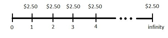
You are considering the purchase of a stock that pays a $2.50 dividend. The dividend is expected to stay constant for the foreseeable future. Assuming a 10% required return, what is the stock worth to you today?

We can start by forecasting the dividends (step one – forecast all expected cash flows). Since the dividends are expected to stay constant for the foreseeable future, this is straightforward as they do not change, so our timeline will look like this:

Note that this is just a perpetuity (infinite annuity) which we introduced in our Time Value of Money Chapter.  Remember that the formula for a perpetuity is

[latex]PV=\frac{PMT}{k}[/latex]

We are going to use the same formula, but just change the notation to reflect stocks so it is:

[latex]P_{0}=\frac{D}{k}[/latex]

Our dividend (D) is $2.50 and our required return (k) is 10% (remember that we need to enter that into the formula as 0.10 and not 10). So, this will give us

[latex]P_{0}=\frac{\$2.50}{0.10}=\$25[/latex]

Example Two

Your firm is planning to raise $2,000,000 by issuing 5% preferred stock with a $40 par value. You anticipate that investors will have a 7% required return. How many shares must you issue if there are no issuance costs? What if the investment banking firm that helps us issue the shares charges us 4% of all proceeds?

While the no growth model (detailed above in example two) is rarely appropriate for common stock (as most companies do not pay out constant dividends over time), it is a good match for preferred stock. Since preferred stock tends to pay a constant dividend (as a percentage of par), it follows the no growth model. Here we need to (a) figure out how much we would receive per share and then (b) how many shares we would need to sell to receive $2,000,000.

[latex]P_{0}=\frac{Par Value * Dividend Rate}{k}=\frac{\$40*0.05}{0.07}=\frac{\$2.00}{0.07}=\$28.57[/latex]

Assuming we can issue shares for $28.57, we would need to issue 70,004 shares ($2,000,000/$28.57) in order to raise $2,000,000.

If the investment banking firm charges us a 4% fee, then we will only get to keep 96% of our proceeds. This means that if we issue shares for $28.57, $1.14 would go to the investment bankers and $27.43 would go to us. So, we now would need to issue 72,913 shares ($2,000,000/$27.43) in order to raise our $2,000,000.

Example Three

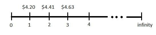
You are considering the purchase of a stock that just paid a dividend (D₀) of $4.00 per share. You forecast that dividends will grow at 5% per year for the foreseeable future. Assuming a 9.5% required return, what is the most that you’d be willing to pay for this stock today?

This no longer fits the no-growth model, so we need to go back to the 3-step valuation process where step one is to forecast all the expected cash flows. Here, we need to introduce the formula to allow us to forecast dividends based on a given growth rate.

[latex]D_{1}=D_{0}(1+g)[/latex]

So, applying this, we get the following:

[latex]D_{1}=\$4.00*(1+0.05)=\$4.20[/latex]

[latex]D_{2}=\$4.20*(1+0.05)=\$4.41[/latex]

[latex]D_{3}=\$4.41*(1+0.05)=\$4.63[/latex]

The problem here is that because the timeline extends to infinity, we would never be able to stop forecasting dividends (note that all our stock valuation models assume we just missed the initial dividend – D₀ – so it is not part of our timeline). This is clearly not practical as if we never stop forecasting dividends, we never get beyond step 1 so we can’t determine the value of the stock. Fortunately, mathematics comes to the rescue. Based on the mathematics of infinite series, we can derive a simple formula to solve for present value of this cash flow stream.

[latex]PV=\frac{D_{1}}{(1+k)}+\frac{D_{2}}{(1+k)^2}+\frac{D_{3}}{(1+k)^3}+...+\frac{D_{\infty}}{(1+k)^\infty}=\frac{D_{1}}{(k-g)}[/latex]

So, our constant growth valuation model is simply:

[latex]P_{0}=\frac{D_{1}}{k-g}[/latex]

Where D₁ is the forecasted dividend for next year, k is the required return (as a decimal) and g is the constant growth rate (also as a decimal).  Applying this model to our example problem gives us:

[latex]P_{0}=\frac{D_{1}}{k-g}=\frac{\$4.00*(1+0.05)}{0.095-0.05}=\frac{\$4.20}{0.045}=\$93.33[/latex]

In addition to just calculating the price like we do in this example, we can also use this model to look at what things influence stock prices. This is actually the strength of the model. Because few firms grow at a constant rate, it is not a very accurate guide to determining how much you should pay for a stock (the non-constant model introduced shortly is much better for that). However, it is a good tool for understanding what causes stock prices to rise or fall.

Stock Prices and Growth Rates

What happens when the growth rate increases from 5% to 6%? How about when it falls from 5% to 3%?

[latex]P_{0}=\frac{D_{1}}{k-g}=\frac{\$4.00*(1+0.06)}{0.095-0.06}=\frac{\$4.24}{0.035}=\$121.14[/latex]

[latex]P_{0}=\frac{D_{1}}{k-g}=\frac{\$4.00*(1+0.03)}{0.095-0.03}=\frac{\$4.12}{0.065}=\$63.38[/latex]

Note that when the growth rate goes up, so does the stock price (from $93.33 with a 5% constant growth rate to $121.14 at a 6% constant growth) and when the growth rate goes down, the stock price falls (from $93.33 with a 5% constant growth rate to $63.38 with a 3% constant growth rate). Stock prices are very sensitive to investors’ forecasted growth rates. When companies announce that they anticipate their growth rates will be slower than previously expected, their stock prices will fall (and sometimes dramatically). The opposite is also true ⇒ increasing growth rates can be a major boost for stock prices. This makes sense from a present value of cash flows basis. If company is growing faster, that means the cash flow stream will get larger faster and increase the present value. If you go all the way back to chapter one, this increases the magnitude of expected cash flows AND improves the timeliness of expected cash flows (again…the cash flows are getting larger at a faster rate).

Stock Prices and Required Returns

What happens when the required return increases from 9.5% to 12%? How about when it falls to 8%?

[latex]P_{0}=\frac{D_{1}}{k-g}=\frac{\$4.00*(1+0.05)}{0.12-0.05}=\frac{\$4.20}{0.07}=\$60.00[/latex]

[latex]P_{0}=\frac{D_{1}}{k-g}=\frac{\$4.00*(1+0.05)}{0.08-0.05}=\frac{\$4.20}{0.03}=\$140.00[/latex]

Note that when the required return goes up, the stock price falls (from $93.33 with a 9.5% required return to $60 with a 12% required return). Alternatively, when the required return goes down (from 9.5% to 8%), the stock price goes up (from $93.33 to $140). Therefore, stock prices are inversely related to changes in the required return (just like bonds). Now, let’s carry this a step further and look at what might lead to increases in the required return for a stock.

• Higher interest rates – as interest rates on bonds increase that means stocks will need to also offer higher returns to stay competitive. For example, if the current interest rate on bonds (which are less risky than stocks) is 6% and the required return for a stock is 8%, what happens when the interest rate on bonds rises to 8%? Now, no one wants the riskier stock for the same return, so the required return on the stock needs to rise to stay attractive to risk-averse investors. Therefore, all else equal, higher interest rates should cause stock prices to fall.
• Higher risk levels – If the risk for a particular stock (or the market as a whole) increases, the required return needs to increase as well due to the concept of risk aversion. Higher risks require higher returns to compensate investors.
• Increased risk aversion – In some cases, risk itself doesn’t need to increase for the required return to rise, just the sensitivity of investors to risk. If investors become more risk-averse as a group, then they will need higher levels of return to compensate them for taking on the risk associated with stocks than they needed previously.

Note that all of the examples here reflected increases in the required return (leading to dropping stock prices), but the opposites hold as well ⇒ lower interest rates, lower risk levels and/or decreased risk aversion should cause required returns to drop and stock prices to go up. Also note that often times it may be a bit harder to see the clear direction if multiple things are changing at the same time. For example, higher interest rates should (all else equal) lead to lower stock prices. However, often higher interest rates may be a result of a stronger economy which could cause investors to revise their growth rates upward (creating upward pressure on the stock price) at the same time as increasing their required return (creating downward pressure on the stock price) and it won’t be clear which will have the greater impact.

Consider the financial crisis of 2008-09. In the summer of 2008, it started to become apparent that many of the large financial institutions were struggling. By the fall of 2008, it became a full-blown crisis that continued to magnify until the spring of 2009 (by January/February 2009, many people were acting as if we were going to be living in something resembling a post-apocalyptic movie very shortly). As a result of this, stock prices dropped dramatically (losing about 50% of their value from their peak prices in 2007). If we look at this through the lens of the stock pricing model above, it makes sense. The collapse of many financial institutions led to a drastic slowdown in the global economy which caused investors to lower their forecasted growth rates. At the same time, the risk of a complete meltdown became more likely, increasing risk and required returns. Finally, investors who were watching the stock market drop regularly (and often very sharply) started to become more risk-averse and increased the required return they felt was necessary to compensate them for owning stocks. All of these things caused stock prices to fall. Then, in the spring of 2009 (about the 2nd week of March), something started to turn around and the growth rates in the global economies went from negative back to positive. The risk of financial meltdown started to appear less likely. Investors saw stock prices didn’t have to fall every day so they became a little less risk-averse. All of these things caused stock prices to rise back up.

Whenever you think of how things are going to impact stock prices think of them in terms of how they are going to impact growth rates and required returns (either for individual firms or the entire market). Be careful not to think of just whether or not the news is good/bad for growth rates and/or required returns, but how the news causes us to revise our expectations for these variables. For instance, news that the economy is expected to decline at 1% when it was expected to decline at 3% is good (growth rate is less negative than expected). Alternatively, news the economy is expected to grow at 4% when it was expected to grow at 6% is bad (growth is less positive than expected). Understanding what drives stock prices is one of the key benefits of the constant growth model.

Example 4

You are evaluating a stock and after doing some research have developed the following information and forecasts. The stock has just paid a dividend of $2.20. You anticipate that the firm will suffer negative growth initially due to problems in the economy and development of some new products. However, after a short down-turn, the growth should explode upward for a brief period before cooling back down. Specifically, you have made the following growth rate forecasts:

Year 1 = -25%
Year 2 = -10%
Year 3 = 50%
Year 4 = 150%
Year 5 = 60%
Year 6 = 30%
Year 7 = 15%
Years 8-infinity = 4%

You anticipate that this is a relatively high risk stock, so feel that a 16% required return is appropriate. Based on this, what is the stock worth today?

While the constant growth model is an improvement on the no-growth model for common stocks, it is still flawed as it assumes that firms grow at the same rate every year forever. This is quite unrealistic. Instead, firms grow fast sometimes (good new products, initial stages of their life cycle, high periods of growth in the economy, etc.) and slow (or even at negative) rates at other times (periods where the firm is poorly managed, new competition enters the field, markets get saturated, new product introductions flop, economic recessions, etc.). Therefore, we need a model that allows for growth rates to vary over time. We will introduce the non-constant (or sometimes called “supernormal”) growth model. Note that we are still using the same 3-step valuation process introduced at the beginning of this handout as the framework, but we are (a) breaking step one into two parts – forecasting dividends and forecasting a terminal value – and (b) we are given the required return so we didn’t include “choose an appropriate discount rate” as a separate step.

Step 1: Forecast dividends up to and including the first year of constant growth

D1 = $2.20*(1 + -0.25) = $2.20*(0.75) = $1.65
D2 = $1.65*(1 + -0.10) = $1.65*(0.90) = $1.49 ⇒ Note round to the nearest cent
D3 = $1.49*(1 + 0.50) = $1.49*(1.50) = $2.24
D4 = $2.24*(1 + 1.50) = $2.24*(2.50) = $5.60
D5 = $5.60*(1 + 0.60) = $5.60*(1.60) = $8.96
D6 = $8.96*(1 + 0.30) = $8.96*(1.30) = $11.65
D7 = $11.65*(1 + 0.15) = $11.65*(1.15) = $13.40
D8 = $13.40*(1 + 0.04) = $13.40*(1.04) = $13.94 ⇒ Note we stop forecasting here as
constant growth is reached

Let us add a few comments on this process.

First, remember that we said a flaw of the constant growth model was that it assumed (unrealistically) that growth rates would grow at the same rate forever. However, what happens when we hit year 8? We assume a constant growth rate. If it is unrealistic today, it is equally unrealistic 8 years from now, so why is it better here? The answer is twofold. First, we have delayed the error by 8 years, so (once discounted back to today) it will have less impact on our final answer. Second, we can’t keep forecasting forever and it is unrealistic to assume we will be able to make good forecasts about year-to-year growth rates several years into the future. Therefore, we forecast as far as we reasonably can and then just assume a constant growth rate for the remaining years, knowing it is only an approximation.

Second, in this example, it is also not very realistic to assume that we know the exact growth rates 6 or 7 years from now. However, what we are doing is just allowing growth to gradually slow from the peak growth in year 4 to the constant growth in year 8 which is probably more realistic than assuming it instantly drops to a constant rate.

Three, when you get to your constant growth rate it should probably be something in the low single digits. It is unrealistic to assume growth of 10-15% per year forever. If that happened, essentially the company would take over the global economy in 100 years. Instead, we see firms grow fast for awhile and then slow down as (a) competition, (b) technological changes, (c) market saturation, (d) poor management, or (e) some combination of the above slows growth down. Reasonable levels for the constant growth rate should probably be in the 0-5% range.

Four, while we stop forecasting dividends at the constant growth stage, it is important to remember that dividends don’t stop here. Instead they keep growing at a constant rate. So, while we stopped forecasting at D₈, there is a D₉, D₁₀, D₁₁, etc.

Step 2: Use the constant growth model to find the value of all remaining dividends at the beginning of the constant growth stage

Because dividends keep going during the constant growth stage, we are going to use the constant growth model to figure out the value of these dividends as of the start of the constant growth stage. Think of two timelines at this point – one that covers years 0 through 7 and a second that covers years 7 through infinity.

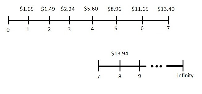
If we look only at the second timeline, this is just a constant growth with D₈ replacing D₁. Since the constant growth model normally uses D₁ to get the price today (P₀), when we substitute D₈ in, it will give us the price in year 7. So,

[latex]P_{7}=\frac{D_{8}}{k-g}=\frac{\$13.94}{0.16-0.04}=\$116.17[/latex]

Step 3: Solve for PV

We are now ready for the last step, solving for the present value of the expected cash flows. To help us visualize this, let’s put all the cash flows on one final timeline.

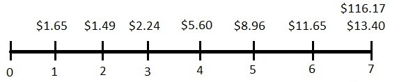
Note that in year 7 there are two separate cash flows. First, we have the dividend in year 7 ($13.40) and second, we have the value of all the remaining dividends from years 8 through infinity ($116.17). Since both of these are year 7 cash flows, before we put them into our financial calculator we have to add them together so that our year 7 cash flow is $129.57 ($13.40 + $116.17). Now, we just put them into our financial calculator (presented below for each of the three calculators).

Table: Calculator Steps for NPV