29 AI-Speak: Deep Neural Networks

Machine learning goes deep

Human knowledge is wide and variable and is inherently difficult to capture. The human mind can absorb and work with knowledge because it is, as Chomsky put it, “a surprisingly efficient and even elegant system that operates with small amounts of information; it seeks not to infer brute correlations among data points but to create explanations¹.”

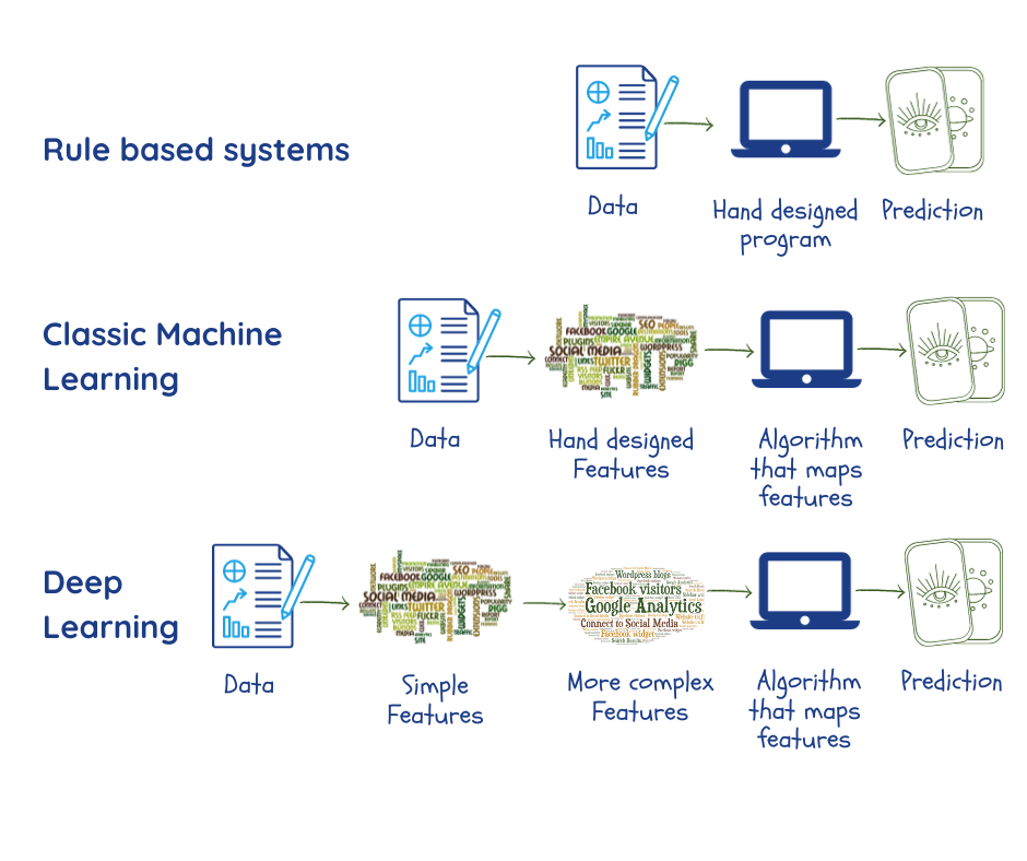
Machine learning is supposed to do it by finding patterns in large amounts of data. But, prior to that, experts and programmers had to sit and code what features of the data are relevant to the problem at hand, and feed these to the machine as “parameters”^2,3. As we saw before, the performance of the system depends heavily on the quality of the data and parameters, which are not always straightforward to pinpoint.

Deep neural networks or deep learning is a branch of machine learning that is designed to overcome this by:

• Extracting its own parameters from data during the training phase;
• Using multiple layers which construct relationships between the parameters, going progressively from simple representations in the outermost layer to more complex and abstract. This enables it to do certain things better than conventional ML algorithms².

Increasingly, most of the powerful ML applications use deep learning. These include search engines, recommendation systems, speech transcription and translation that we have covered in this book. It will not be a stretch to say that deep learning has propelled the success of artificial intelligence in multiple tasks.

“Deep” refers to how the layers pile on top of each other to create the network. “Neural” reflects the fact that some aspects of the design were inspired by the biological brain. Despite that, and even though they provide some insights into our own thought processes, these are strictly mathematical models and do not resemble any biological parts or processes².

The basics of deep learning

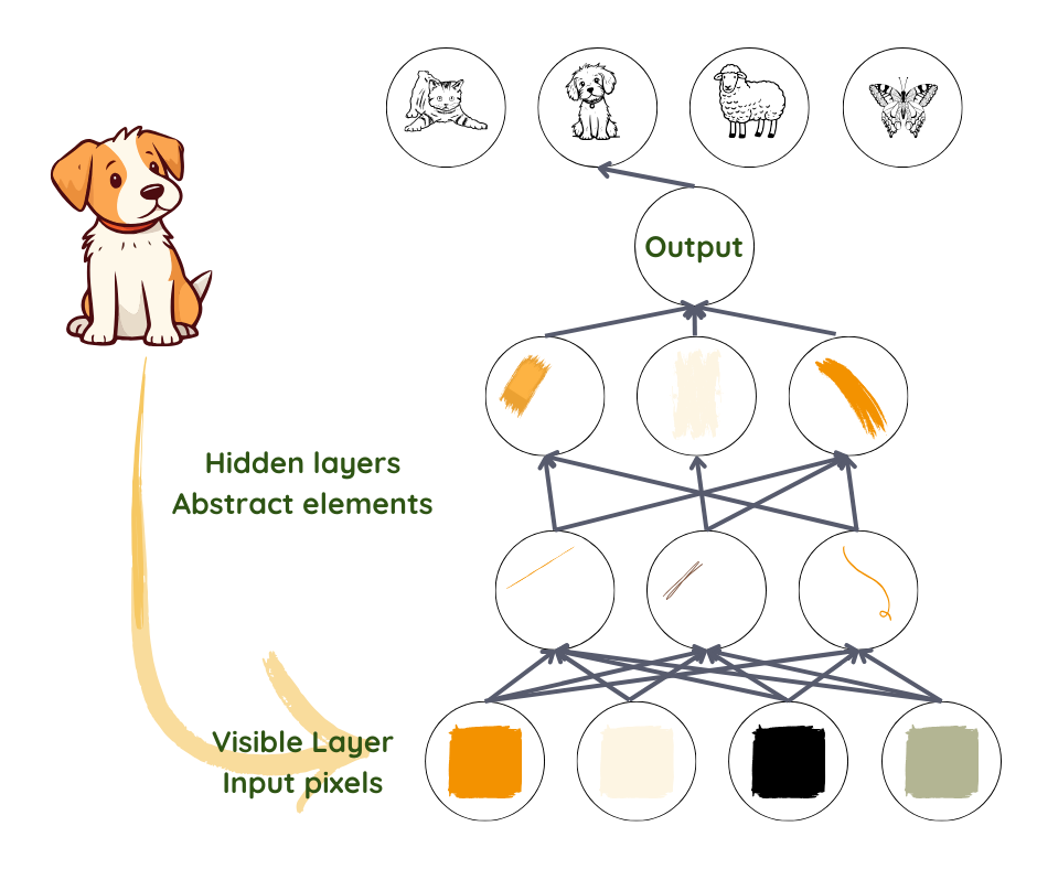
When humans look at a picture, we automatically identify objects and faces. But a photo is just a collection of pixels for an algorithm. Going from a jumble of colours and brightness levels, to recognising a face, is a leap too complicated to execute.

Deep learning achieves this by breaking the process into simple representations in the first layer – by, say, comparing brightness of neighbouring pixels to note the presence or absence of edges in various regions of the image. The second layer takes collections of edges to search for more complex entities – such as corners and contours, ignoring small variations in edge positions^2,3. The next layer looks for parts of the objects using the contours and corners. Slowly, the complexity builds till the point where the last layer can combine different parts well enough to recognise a face or identify an object.

.

What to take into account in each layer is not specified by programmers but is learned from data in the training process3. By testing these predictions with the real outputs in the training dataset, the functioning of each layer is tuned in a slightly different way to get a better result each time. When done correctly, and provided there is sufficient good-quality data, the network should evolve to ignore irrelevant parts of the photo, like exact location of the entities, angle and lighting, and zero in on those parts which make recognition possible.

Of note here is the fact that, despite our use of edges and contours to understand the process, what is actually represented in the layers is a set of numbers, which might or might not correspond to things that we understand. What doesn’t change is the increasing abstractness and complexity.

Designing the network

Once the programmer decides to use deep learning for a task and prepares the data, they have to design what is called the architecture of their neural network. They have to choose the number of layers (depth of the network) and the number of parameters per layer (width of the network). Next, they have to decide how to make connections between the layers – whether or not each unit of a layer will be connected to every unit of the previous layer.

The ideal architecture for a given task is often found by experimentation. The greater the number of layers, the fewer the parameters that are needed per layer and the network performs better with general data, at the cost of it being difficult to optimise. Fewer connections would mean fewer parameters, and lesser amount of computation, but reduces the flexibility of the network².

Training the network

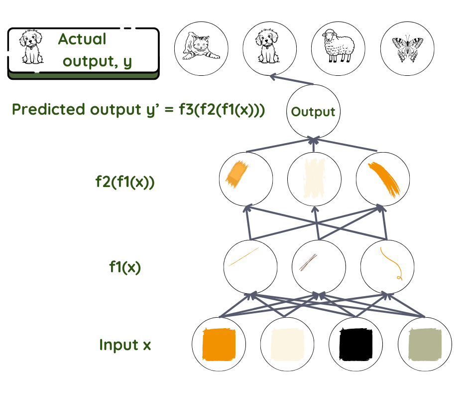
Let us take the example of a feed forward neural network doing supervised learning. Here, information flows forward from layer to deeper layer, with no feedback loops. As for all machine-learning techniques, the goal here is to find out how the input is connected to the output – what parameters come together, and how they come together to give the observed result. We assume a relationship f that connects the input x to the output y. We then use the network to find the set of parameters θ that give the best match for predicted and actual outputs.

Here the prediction for y is the final product and the dataset x is the input. In face recognition, x is usually the set of pixels in an image. y can be the name of the person. In the network, the layers are like workers in an assembly line, where each worker works on what is given to them and passes it forward to the next worker. The first one takes the input and transforms it a little bit and gives it to the second in line. The second does the same before passing it to the third, and so on until the input is transformed into the final product.

Mathematically, the function f is split into many functions f1, f2, f3… where f= ….f3(f2(f1(x))). The layer next to the input transforms input parameters using f1, the next layer using f2, and so on. The programmer might intervene to help choose the correct family of functions based on their knowledge of the problem.

It is the work of each layer to assign the level of importance – the weight given to each parameter that it receives. These weights are like knobs that ultimately define the relationship between the predicted output and input in that layer³. In a typical deep-learning system, we are looking at hundreds of millions of these knobs and hundreds of millions of training examples. Since we neither define nor can see the output and weights in the layers between input and output, these are called hidden layers.

In the case of the object recognition example discussed above, it is the work of the first worker to detect edges and pass on the edges to the second one who detects contours and so on.

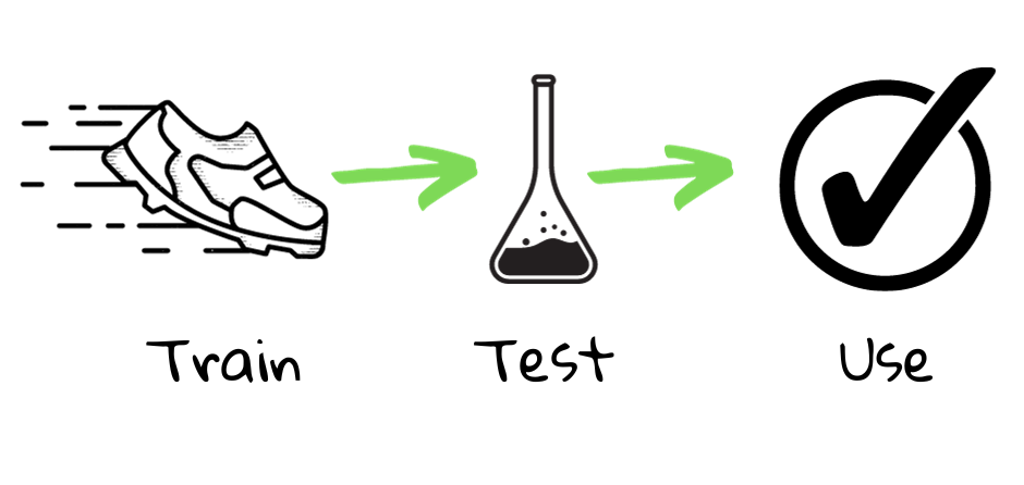
During training, the predicted output is taken and compared with the real output. If there is a big difference between the two, the weights assigned in each layer will have to be changed by a lot. If not, they have to be changed a little. This work is done in two parts. First the difference between prediction and output is calculated. Then another algorithm computes how to change the weights in each layer, starting from the output layer (in this case, the information flows backwards from the deeper layers). Thus at the end of the training process, the network is ready with its weights and functions to attack test data. The rest of the process is the same as that of conventional machine learning.

¹ Chomsky, N., Roberts, I., Watumull, J., Noam Chomsky: The False Promise of ChatGPT, The New York Times, 2023.

² Goodfellow, I.J., Bengio, Y., Courville, A., Deep Learning, MIT Press, 2016.

³ LeCun, Y., Bengio, Y., Hinton, G., Deep learning, Nature 521, 436–444 (2015).