APPLICATIONS

Alicia Y. Tsai; Authors: Laurent EI Ghaoui; Contributors: Phan Hoang, Tony Tin, Ha To Tam, Nguyen Van Kep, Le Dinh Nam, Juliette Decugis, Nguyen Quoc Cuong.; Giuseppe C. Calafiore

26 APPLICATIONS

26.1. Linear regression via least-squares

Linear regression is based on the idea of fitting a linear function through data points.

In its basic form, the problem is as follows. We are given data $(y_i, x_i), i=1, \ldots, m$ where $x_i \in \mathbb{R}^n$ is the ‘‘input’’ and $y_i \in \mathbb{R}$ is the ‘‘output’’ for the $i-$ th measurement. We seek to find a linear function $f: \mathbb{R}^n \to \mathbb{R}$ such that $f(x_i)$ are collectively close to the corresponding values $y_i$ .

In least-squares regression, the way we evaluate how well a candidate function $f$ fits the data is via the (squared) Euclidean norm:

$\sum_{i=1}^m\left(y_i-f\left(x_i\right)\right)^2 .$

Since a linear function $f$ has the form $f(x)=\theta^T x$ for some $\theta \in \mathbb{R}^n$ , the problem of minimizing the above criterion takes the form

$\min _\theta \sum_{i=1}^m\left(y_i-x_i^T \theta\right)^2 .$

We can formulate this as a least-squares problem:

$\min _\theta\|A \theta-y\|_2,$

where

$A=\left(\begin{array}{c} x_1^T \\ \vdots \\ x_m^T \end{array}\right)$

The linear regression approach can be extended to multiple dimensions, that is, to problems where the output in the above problem contains more than one dimension (see here). It can also be extended to the problem of fitting non-linear curves.

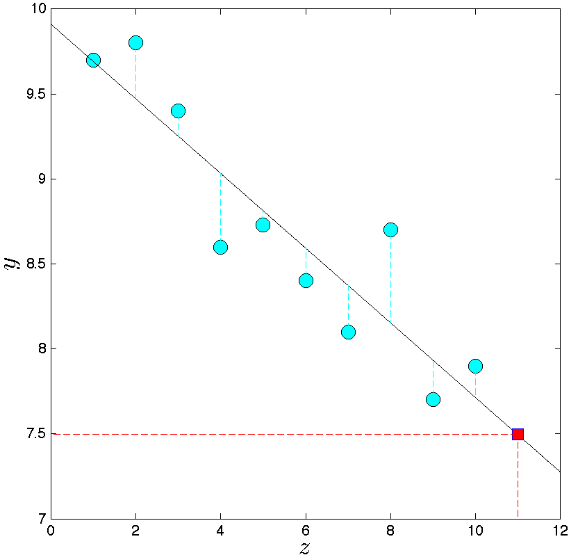	In this example, we seek to analyze how customers react to an increase in the price of a given item. We are given two-dimensional data points $\left(x_i, y_i\right), i=1, \ldots, m$ . The $x_i$ ‘s contain the prices of the item, and the $y_i$ ‘s the average number of customers who buy the item at that price.
	The generic equation of a non-vertical line is $y=\theta_1 x+\theta_2$ , where $\theta=\left(\theta_1, \theta_2\right)$ contains the decision variables. The quality of the fit of a generic line is measured via the sum of the squares of the error in the component $y$ (blue dotted lines). Thus, the best least-squares fit is obtained via the least-squares problem
	$\min _\theta \sum_{i=1}^m\left(\theta_1 x_i+\theta_2-y_i\right)^2 .$
	Once the line is found, it can be used to predict the value of the average number of customers buying the item ( $y$ ) for a new price ( $x$ ). The prediction is shown in red.

See also: The problem of Gauss.

26.2. Auto-regressive models for time-series prediction.

A popular model for the prediction of time series is based on the so-called auto-regressive model

$y_t=\theta_1y_{t-1}+\ldots+\theta_my_{t-m}, \quad t=1,\ldots,m,$

where $\theta_i$ ‘s are constant coefficients, and $m$ is the ‘‘memory length’’ of the model. The interpretation of the model is that the next output is a linear function of the past. Elaborate variants of auto-regressive models are widely used for the prediction of time series arising in finance and economics.

To find the coefficient vector $\theta=(\theta_1, \ldots, \theta_m)$ in $\mathbb{R}^m$ , we collect observations $\left(y_t\right)_{0 \leq t \leq T}$ (with $T \geq m$ ) of the time series, and try to minimize the total squared error in the above equation: