• Image compression.
• Market data analysis.

39.1 Image compression

Images as matrices

We can represent images as matrices, as follows. Consider an image having pixels. For gray scale images, we need one number per pixel, which can be represented as a matrix. For color images, we need three numbers per pixel, for each color: red, green, and blue (RGB). Each color can be represented as a matrix, and we can represent the full color image as a matrix, where we stack each color’s matrix column-wise alongside each other, as

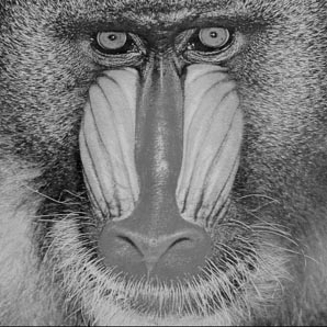The image on the left is a grayscale image, which can be represented as a matrix containing the gray scale values stored as integers.

The image can be visualized as well. We must first transform the matrix from integer to double. In JPEG format, the image will be loaded into matlab as a three-dimensional array, one matrix for each color. For gray scale images, we only need the first matrix in the array.

Low-rank approximation

Using the low-rank approximation via SVD method, we can form the best rank- approximations for the matrix.

True and approximated images, with varying rank. We observe that with , the approximation is almost the same as the original picture, whose rank is .

Recall that the explained variance of the rank- approximation is the ratio between the squared norm of the rank- approximation matrix and the squared norm of the original matrix. Essentially, it measures how much information is retained in the approximation relative to the original.

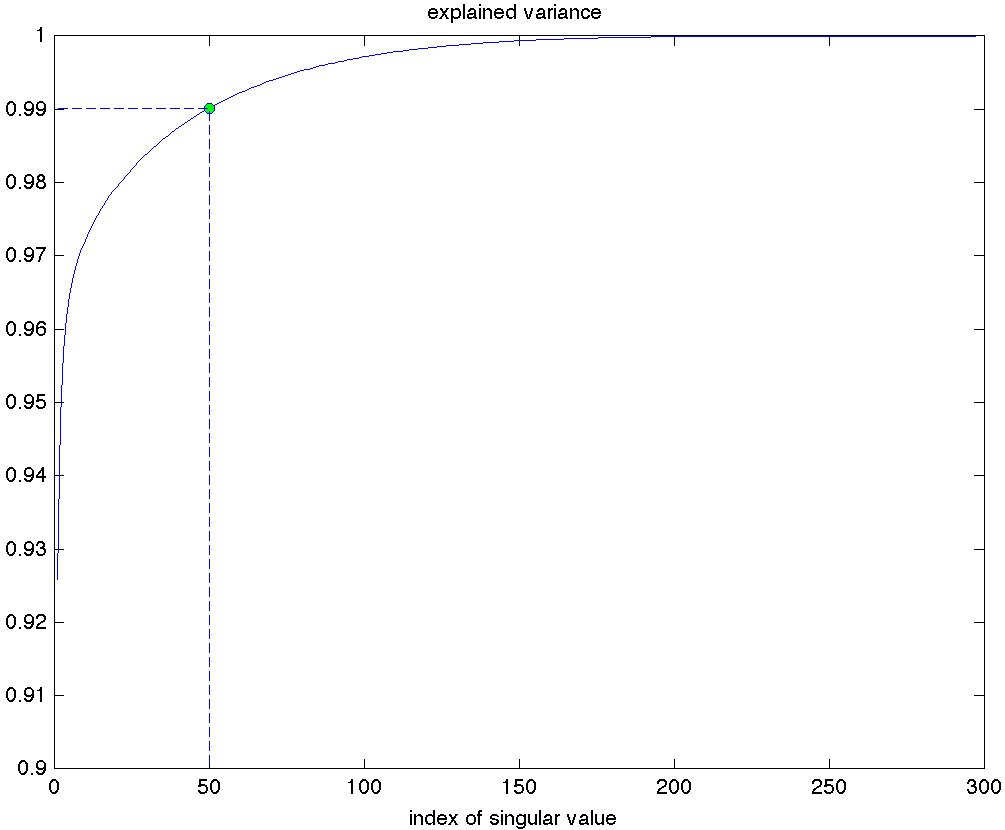The explained variance for the various rank- approximations to the original image provides insight into the fidelity of the approximation. For , the approximation contains more than 99% of the total variance in the picture, suggesting that the rank-50 approximation is almost indistinguishable from the original in terms of information content.

39.2 Market data analysis

We consider the daily log-returns of a collection of stocks chosen in the Fortune 100 companies over the time period from January 3, 2007, until December 31, 2008. We can represent this as a matrix, with each column a day, and each row a time-series corresponding to a specific stock.

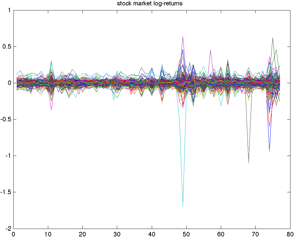The image on the left represents the time series of the stock market mentioned above, shown as a collection of time-series. We note that the log-returns hover around a mean which appears to be close to zero.

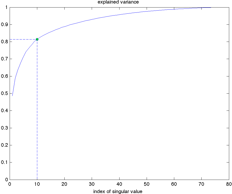We can form the SVD of the matrix of log-returns and plot the explained variance. We see that the first 10 singular values explain more than 80% of the data’s variance.

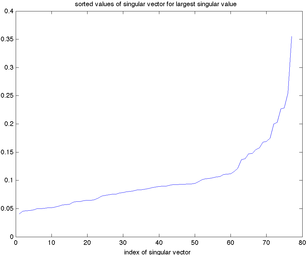
It is instructive to look at the singular vector corresponding to the largest singular value, arranged in increasing order. We observe that all the components have the same sign (which we can always assume is positive). This means we can interpret this vector as providing a weighted average of the market. As seen in the previous plot, the corresponding rank-one approximation roughly explains more than 80% of the variance in this market data, which justifies the phrase ‘‘the market average moves the market’’. The five components with largest magnitude correspond to the following companies. Note that all are financial:

• FABC (Fidelity Advisor)
• FTU (Wachovia, bought by Wells Fargo)
• MER (Merrill Lynch, bought by Bank by America)
• AIG (don’t need to elaborate)

• MS (Morgan Stanley)