APPLICATIONS: PCA OF SENATE VOTING DATA

Alicia Y. Tsai; Authors: Laurent EI Ghaoui; Contributors: Phan Hoang, Tony Tin, Ha To Tam, Nguyen Van Kep, Le Dinh Nam, Juliette Decugis, Nguyen Quoc Cuong.; Giuseppe C. Calafiore

32 APPLICATIONS: PCA OF SENATE VOTING DATA

32.1 Introduction

In this case study, we take data from the votes on bills in the US Senate (2004-2006) and explore how we can visualize the data by projecting it, first on a line then on a plane. We investigate how we can choose the line or plane in a way that maximizes the variance in the result, via a principal component analysis method. Finally, we examine how a variation on PCA that encourages sparsity of the projection directions allows us to understand which bills are most responsible for the variance in the data.

32.2. Senate voting data and the visualization problem

Data

The data consists of the votes of $n=100$ Senators in the 2004-2006 US Senate (2004-2006), for a total of $m=542$ bills. “Yay” (“Yes”) votes are represented as $1$ ‘s, “Nay” (“No”) as $-1$ ‘s, and the other votes are recorded as $0$ . (A number of complexities are ignored here, such as the possibility of pairing the votes.)

This data can be represented here as a $m \times n$ ‘‘voting’’ matrix $X = [x_1,\ldots,x_n]$ , with elements taken from $\{-1,0,1\}$ . Each column of the voting matrix $x_j$ , $j=1,\ldots,n$ contains the votes of a single Senator for all the bills; each row contains the votes of all Senators on a particular bill.

Senate voting matrix: “Nay” votes are in black, “Yay” ones in white, and the others in grey. The transpose voting matrix is shown. The picture becomes has many gray areas, as some Senators are replaced over time. Simply plotting the raw data matrix is often not very informative.

Visualization Problem

We can try to visualize the data set, by projecting each data point (each row or column of the matrix) on (say) a 1D-, 2D- or 3D-space. Each ‘‘view’’ corresponds to a particular projection, that is, a particular one-, two- or three-dimensional subspace on which we choose to project the data. The visualization problem consists of choosing an appropriate projection.

There are many ways to formulate the visualization problem, and none dominates the others. Here, we focus on the basics of that problem.

32.3. Projecting on a line

To simplify, let us first consider the simple problem of representing the high-dimensional data set on a simple line, using the method described here.

Scoring Senators

Specifically we would like to assign a single number, or ‘‘score’’, to each column of the matrix. We choose a direction $u$ in $\mathbb{R}^m$ , and a scalar $v$ in $\mathbb{R}$ . This corresponds to the affine ‘‘scoring’’ function $f : \mathbb{R}^m \rightarrow \mathbb{R}$ , which, to a generic column $x$ in $\mathbb{R}^m$ of the data matrix, assigns the value

$\begin{align*} f(x) = u^T x + v. \end{align*}$

We thus obtain a vector of values $f$ in $\mathbb{R}^n$ , with

$\begin{align*} f_j = u^T x_j + v, \quad j=1,\ldots,n. \end{align*}$

It is often useful to center these values around zero. This can be done by choosing $v$ such that

$\begin{align*} 0 &= \sum_{j=1}^n ( u^T x_j + v ) = u^T \left( \sum_{j=1}^n x_j \right) + n \cdot v, \end{align*}$

that is: $v = -u^T \hat{x},$ where

$\begin{align*} \hat{x} := \frac{1}{n} \sum_{j=1}^n x_j \in \mathbb{R}^m \end{align*}$

is the vector of sample averages across the columns of the matrix (that is, data points). The vector $\hat{x}$ can be interpreted as the ‘‘average response’’ across experiments.

The values of our scoring function can now be expressed as

$\begin{align*} f(x) = u^T (x-\hat{x}). \end{align*}$

In order to be able to compare the relative merits of different directions, we can assume, without loss of generality, that the vector $u$ is normalized (so that $||u||_2 = 1$ ).

Centering data

It is convenient to work with the ‘‘centered’’ data matrix, which is

$\begin{align*} X_{\text{cent}} = \left( \begin{array}{ccc} x_1 -\hat{x} & \ldots & x_n - \hat{x} \end{array}\right) = X - \hat{x}\mathbf{1}_n^T, \end{align*}$

where $\mathbf{1}_n$ is the vector of ones in $\mathbb{R}^n$ .

We can compute the (row) vector scores using the simple matrix-vector product:

$\begin{align*} f = u^T X_{\text{cent}} \in \mathbb{R}^{1 \times m}. \end{align*}$

We can check that the average of the above row vector is zero:

$\begin{align*} f\mathbf{1}_n = u^T X_{\text{cent}}\mathbf{1}_n = u^T(X - \hat{x}\mathbf{1}_n^T) \mathbf{1}_n = u^T(X\mathbf{1}_n - n \cdot \hat{x}) = 0. \end{align*}$

Example: visualizing along random direction

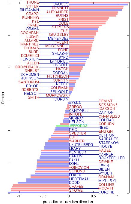Scores obtained with random direction: This image shows the values of the projections of the Senator’s votes $x_j-\hat{x}$ (that is, with average across Senators removed) on a (normalized) ‘‘random bill’’ direction. This projection shows no particular obvious structure. Note that the range of the data is much less than obtained with the average bill shown above.

32.4. Projecting on a plane

We can also try to project the data on a plane, which involves assigning two scores to each data point.

Scoring Map

This corresponds to the affine ‘‘scoring’’ map $f : \mathbb{R}^m \rightarrow \mathbb{R}$ , which, to a generic column $x$ in $\mathbb{R}^m$ of the data matrix, assigns the two-dimensional value

$f(x) = \left( \begin{array}{c} u_1^Tx + v_1 \\ u_2^Tx+v_2 \end{array}\right) = U^Tx + v,$

where $u_1,u_2 \in \mathbb{R}^m$ are two vectors, and $v_1,v_2$ two scalars, while $U = [u_1,u_2] \in \mathbb{R}^{m \times 2}$ , $v \in \mathbb{R}^2$ .

The affine map $f$ allows to generate $n$ two-dimensional data points (instead of $m$ -dimensional) $f_j = U^Tx_j+v$ , $j=1,\ldots,n$ . As before, we can require that the $f_j's$ be centered:

$0 = \sum_{j=1}^n f_j = \sum_{j=1}^n (U^Tx_j+v) ,$

by choosing the vector $v$ to be such that $v = -U^T\hat{x}$ , where $\hat{x} \in \mathbb{R}^m$ is the ‘‘average response’’ defined above. Our (centered) scoring map takes the form

$f(x) = U^T(x-\hat{x}).$

We can encapsulate the scores in the $2 \times n$ matrix $F=[f_1,\ldots,f_n]$ . The latter can be expressed as the matrix-matrix product

$F = U^TX_{\text{cent}} = \left( \begin{array}{c} u_1^TX_{\text{cent}} \\ u_2^TX_{\text{cent}} \end{array}\right),$

with $X_{\text{cent}}$ the centered data matrix defined above.

Clearly, depending on which plan we choose to project on, we get very different pictures. Some planes seem to be more ‘‘informative’’ than others. We return to this issue here.

Two-dimensional projection of the Senate voting matrix: This particular projection does not seem to be very informative. Notice in particular, the scale of the vertical axis. The data is all but crushed to a line, and even on the horizontal axis, the data does not show much variation.

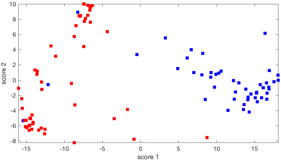Two-dimensional projection of the Senate voting matrix: This particular projection seems to allow to cluster the Senators along party line, and is therefore more informative. We explain how choose such a direction here.

32.5. Direction of maximal variance

Motivation

We have seen here how we can choose a direction in bill space, and then project the Senate voting data matrix on that direction, in order to visualize the data along a single line. Clearly, depending on how we choose the line, we will get very different pictures. Some show large variation in the data, others seems to offer a narrower range, even if we take care to normalize the directions.

What could be a good criterion to choose the direction we project the data on?

It can be argued that a direction that results in large variations of projected data is preferable to a one with small variations. A direction with high variation ‘‘explains’’ the data better, in the sense that it allows to distinguish between data points better. One criteria that we can use to quantify the variation in a collection of real numbers is the sample variance, which is the sum of the squares of the differences between the numbers and their average.

Solving the maximal variance problem

Let us find a direction which maximizes the empirical variance. We seek a (normalized) direction $u$ such that the empirical variance of the projected values $u^Ta_j$ , $j=1,\ldots,n$ , is large. If $\hat{a}$ is the vector of averages of the $a_j$ ‘s, then the average of the projected values is $u^T\hat{a}$ . Thus, the direction of maximal variance is one that solves the optimization problem

$\max_{u : \|u\|_2 = 1} \frac{1}{n} \sum_{j=1}^n \left( (x_j-\hat{a})^Tu \right)^2.$

The above problem can be formulated as

$\max_{u : \|u\|_2 = 1} u^T\Sigma u,$

where

$\Sigma := \frac{1}{n} \sum_{j=1}^n (x_j-\hat{a})(x_j-\hat{a})^T$

is the $m \times m$ sample covariance matrix of the data. The interpretation of the coefficient $\Sigma_{kl}$ is that it provides the covariance between the votes of Senator $k$ and those of Senator $l$ .

We have seen the above problem before, under the name of the Rayleigh quotient of a symmetric matrix. Solving the problem entails simply finding an eigenvector of the covariance matrix $\Sigma$ that corresponds to the largest eigenvalue.


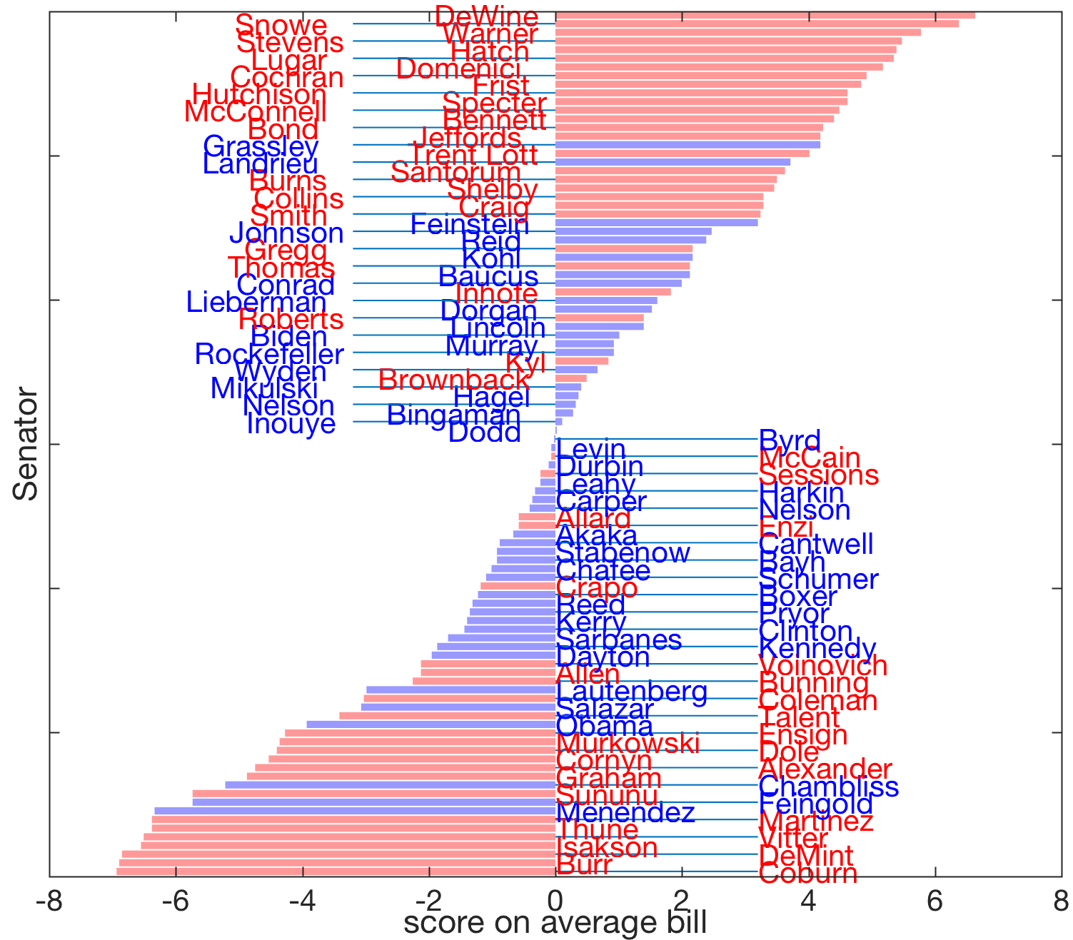	This image shows the scores assigned to each Senator along the direction of maximal variance, $u_{\text{max}}^T(x_j-\hat{x})$ , $j=1,\ldots,n$ , with $u_{\text{max}}$ a normalized eigenvector corresponding to the largest eigenvalue of the covariance matrix $\Sigma$ . Republican Senators tend to score positively, while we find many Democrats on the negative score. Hence the direction could be interpreted as revealing the party affiliation.
	Note that the largest absolute score (about 18) obtained in this plot is about three times bigger than that observed on the previous one. This is consistent with the fact that the current direction has maximal variance.

32.6. Principal component analysis

Main idea

The main idea behind principal components analysis is to first find a direction that corresponds to maximal variance between the data points. The data is then projected on the hyperplane orthogonal to that direction. We obtain a new data set and find a new direction of maximal variance. We may stop the process when we have collected enough directions (say, three if we want to visualize the data in 3D).

Mathematically, the process amounts to finding the eigenvalue decomposition of a positive semi-definite matrix: the covariance matrix of the data points. The directions of large variance correspond to the eigenvectors with the largest eigenvalues of that matrix. The projection to use to obtain, say, a two-dimensional view with the largest variance, is of the form $x \rightarrow Px$ , where $P= [u_1,u_2]^T$ is a matrix that contains the eigenvectors corresponding to the first two eigenvalues.

Low rank approximations

In some cases, we are not specifically interested in visualizing the data, but simply to approximate the data matrix with a ‘‘simpler’’ one.

Assume we are given a (sample) covariance matrix of the data, $\Sigma$ . Let us find the eigenvalue decomposition of $\Sigma$ :

$\Sigma = \sum_{i=1}^m \lambda_i u_i u_i^T = U \textbf{diag}(\lambda_1,\ldots,\lambda_m) U^T,$

where $U$ is an $m \times m$ orthogonal matrix. Note that the trace of that matrix has an interpretation as the total variance in the data, which is the sum of all the variances of the votes of each Senator:

$\textbf{Trace} ( \Sigma ) = \sum_{i=1}^m \lambda_i.$

Now let us plot the values of $\lambda_i$ ‘s in decreasing order.

This image shows the eigenvalues of the $m \times m$ covariance matrix of the Senate voting data, which contains the covariances between the votes of each pair of Senators.

Clearly, the eigenvalues decrease very fast. One is tempted to say that ‘‘most of the information’’ is contained in the first eigenvalue. To make this argument more rigorous, we can simply look at the ratio:

$\frac{\lambda_1}{\lambda_1 + \ldots + \lambda_m}$

which is the ratio of the total variance in the data (as approximated by $\hat{\Sigma}$ ) to that of the whole matrix $\Sigma$ .

In the Senate voting case, this ratio is of the order of 90%. It turns out that this is true of most voting patterns in democracies across history: the first eigenvalue ‘‘explains most of the variance’’.

32.7. Sparse PCA

Motivation

Recall that the direction of maximal variance is one vector $u \in \mathbb{R}^m$ that solves the optimization problem

$\max_{u : \|u\|_2 = 1} \frac{1}{n} \sum_{j=1}^n \left( (x_j-\hat{a})^Tu \right)^2 \Longleftrightarrow \max_{u : \|u\|_2 = 1} u^T\Sigma u, \; \; \text{ where } \Sigma := \frac{1}{n} \sum_{j=1}^n (x_j-\hat{a})(x_j-\hat{a})^T.$

Here $\hat{a} := \frac{1}{n} \sum_{j=1}^n x_j$ is the estimated center. We obtain a new data set by combining the variables according to the directions determined by $u$ . The resulting dataset would have the same dimension as the original dataset, but each dimension has a different meaning (since they are linear projected images of the original variables).

As explained, the main idea behind principal components analysis is to find those directions that corresponds to maximal variances between the data points. The data is then projected on the hyperplane spanned by these principal components. We may stop the process when we have collected enough directions in the sense that the new directions explain the majority of the variance. That is, we can pick those directions corresponding to the highest scores.

We may also wonder if $u$ can have only a few non-zero coordinates. For example, if the optimal direction $u$ is $(0.01, 0.02, 200, 100) \in \mathbb{R}^4$ , then it is clear that the 3rd and 4th bills are characterizing most features, and we may simply want to drop the 1st and 2nd bills. That is, we want to adjust the optimal direction vector as $(0, 0, 200, 100) \in \mathbb{R}^4$ . This adjustment accounts for sparsity. In the setting of PCA analysis, each principal component is linear combinations of all input variables. Sparse PCA allows us to find principal components as linear combinations that contain just a few input variables (hence it looks “sparse” in the input space). This feature would enhance the interpretability of the resulting dataset and perform dimension reduction in the input space. Reducing the number of input variables would assist us in the senate voting dataset, since there are more bills (input variables) than senators (samples).

We are going to compare this result of PCA to sparse PCA results below.



	This image shows the scores assigned to each Senator along the direction of maximal variance, $u^T_{\text{max}}(x_j - \hat{x})$ , $j = 1, \ldots, n$ , with $u_{\text{max}}$ corresponding to the PCA optimization problem. Republican Senators tend to score positively, while we find many Democrats on the negative score. Hence the direction could be interpreted as revealing the party affiliation.
	We are going to compare this result of PCA to sparse PCA results below.

32.8 Sparse maximal variance problem

Main Idea

A mathematical generalization of the PCA can be obtained by modifying the PCA optimization problem above. We attempt to find the direction of maximal variance as one vector $u \in \mathbb{R}^m$ that solves the optimization problem

$\begin{aligned}\max_{u : \|u\|_2 = 1, \|u\|_0 \leq k} \frac{1}{n} \sum_{j=1}^n \left( (x_j-\hat{a})^Tu \right)^2 \Longleftrightarrow \max_{u : \|u\|_2 = 1, \|u\|_0 \leq k} u^T\Sigma u,\end{aligned}$

where

$\Sigma = \frac{1}{n} \sum_{j=1}^n (x_j-\hat{a})(x_j-\hat{a})^T.$

The difference is that we put one more constraint $\|u\|_0 \leq k$ , where $\|u\|_0$ is the number of non-zero coordinates in the vector $u$ . For instance, $\|(0.01, 0.02, 200, 100)\|_0 = 4$ but $\|(0, 0, 200, 100)\|_0 = 2$ . Here, $k$ is a pre-determined hyper-parameter that describes the sparsity of the input space we want. This constraint of $\|u\|_0 \leq k$ makes the optimization problem non-convex, and without an analytically closed solution. But we still have a numerical solution and the sparse properties as we explained. However, $\|u\|_0$ makes the optimization problem non-convex and is difficult to solve. Instead, we practice an $L_1$ regularization relaxation alternative

$\begin{aligned}\max_{u : \|u\|_2 = 1} \frac{1}{n} \sum_{j=1}^n \left( (x_j-\hat{a})^Tu \right)^2 + \lambda \|u\|_1 \Longleftrightarrow \max_{u : \|u\|_2 = 1} u^T\Sigma u + \lambda \|u\|_1.\end{aligned}$

This optimization problem is convex and can be solved numerically; this is the so-called sparse PCA (SPCA) method. The $\lambda$ parameter is a pre-determined hyper-parameter we introduced as a penalty parameter, which can be tuned, as we shall see below.

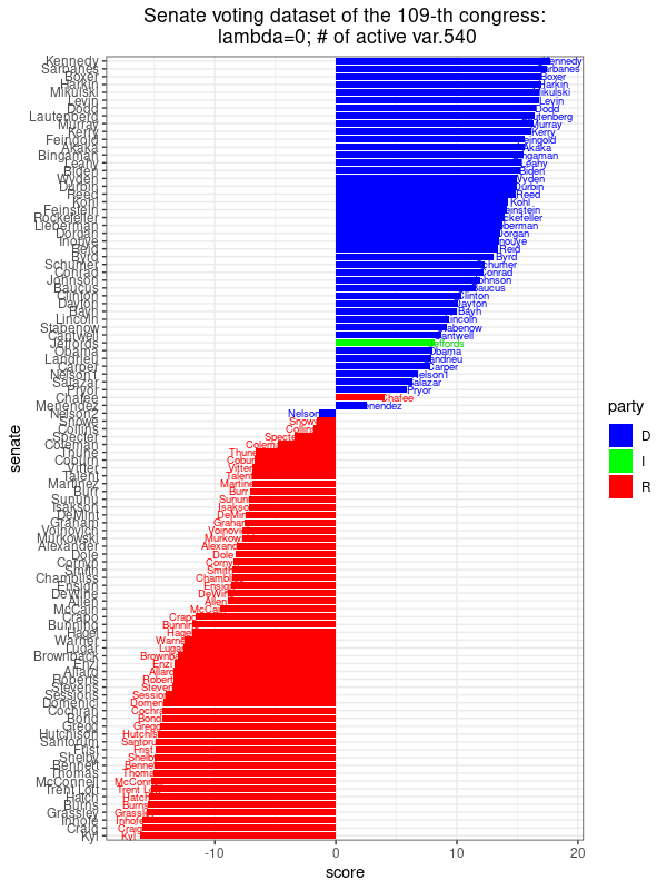
Analysis of the senate dataset

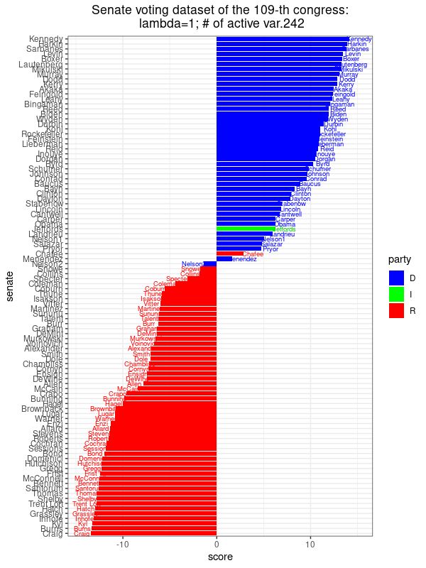
We can apply the SPCA method onto the senate voting dataset, with $\lambda = 0$ (i.e. PCA) and increase $\lambda$ to values of 1, 10, and 1000. In each setting, we also record the number of non-zero coordinates of $u_{\text{max}}$ , which is a solution to the SPCA optimization problem above. Since each coordinate of $u_{\text{max}}$ represents the voting outcome of one bill, we call the number of non-zero coordinates of $u_{\text{max}}$ as the number of active variables. From the results below, we did not observe much change in the separation of party lines given by the principal components. As $\lambda$ increases to 1000, there are only 7 active variables left. The corresponding 7 bills, which are important for distinguishing the party lines of senators, are:

8 Energy Issues LIHEAP Funding Amendment 3808
16 Abortion Issues Unintended Pregnancy Amendment 3489
34 Budget, Spending and Taxes Hurricane Victims Tax Benefit Amendment 3706
36 Budget, Spending and Taxes Native American Funding Amendment 3498
47 Energy Issues Reduction in Dependence on Foreign Oil 3553
59 Military Issues Habeas Review Amendment 3908
81 Business and Consumers Targeted Case Management Amendment 3664



	This image shows the scores assigned to each Senator along the direction of maximal variance, $u_{\text{max}}^T (x_j - \hat{x})$ for $j = 1, \ldots, n$ , where the $u_{\text{max}}$ corresponds to the sparse PCA optimization problem with $\lambda = 1$ . There are 242 non-zero coefficients, meaning that we only need 242 different bills to get this score revealing the party affiliation to this extent. This is almost identical to the result obtained from PCA.



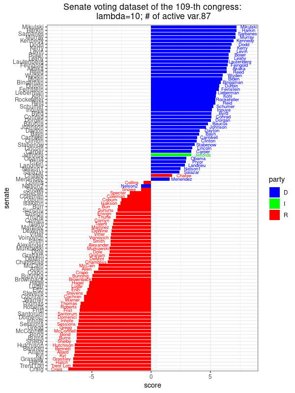
	This image shows the scores assigned to each Senator along the direction of maximal variance, $u_{\text{max}}^T (x_j - \hat{x})$ for $j = 1, \ldots, n$ , where the $u_{\text{max}}$ corresponds to the sparse PCA optimization problem with $\lambda = 10$ . There are 87 non-zero coefficients, meaning that we only need 87 different bills to get this score revealing the party affiliation to this extent. Compared to PCA, there is one more mis-classified senator.



	This image shows the scores assigned to each Senator along the direction of maximal variance, $u_{\text{max}}^T (x_j - \hat{x})$ for $j = 1, \ldots, n$ , where the $u_{\text{max}}$ corresponds to the sparse PCA optimization problem with $\lambda = 1000$ . There are 8 non-zero coefficients, meaning that we only need 8 different bills to get this score revealing the party affiliation to this extent, which is not much different from PCA using all 542 votes as in PCA.

License

Icon for the Creative Commons Attribution-NonCommercial-NoDerivatives 4.0 International License

32.1 Introduction

32.2. Senate voting data and the visualization problem

Data

Visualization Problem

32.3. Projecting on a line

Scoring Senators

Centering data

Example: visualizing along random direction

32.4. Projecting on a plane

Scoring Map

32.5. Direction of maximal variance

Motivation

Solving the maximal variance problem

32.6. Principal component analysis

Main idea

Low rank approximations

32.7. Sparse PCA

Motivation

32.8 Sparse maximal variance problem

Main Idea

Analysis of the senate dataset

License

Share This Book