EXERCISES

Alicia Y. Tsai; Authors: Laurent EI Ghaoui; Contributors: Phan Hoang, Tony Tin, Ha To Tam, Nguyen Van Kep, Le Dinh Nam, Juliette Decugis, Nguyen Quoc Cuong.; Giuseppe C. Calafiore

27 EXERCISES

27.1. Standard forms

Regularization for noisy data. Consider a least-squares problem

$\min _x\|A x-y\|_2^2$

in which the data matrix $A \in \mathbb{R}^{m \times n}$ is noisy. Our specific noise model assumes that each row $a_i^T \in \mathbb{R}^n$ has the form $a_i=\hat{a}_i+u_i$ , where the noise vector $u_i \in \mathbb{R}^n$ has zero mean and covariance matrix $\sigma^2I_n$ , with $\sigma$ a measure of the size of the noise. Therefore, now the matrix $A$ is a function of the set of uncertain vectors $u=\left(u_1, \ldots, u_n\right)$ , which we denote by $A(u)$ . We will write $\hat{A}$ to denote the matrix with rows $\hat{a}_i^T, \; i=1, \ldots, m$ . We replace the original problem with

$\min _x \mathbf{E}_u\|A(u) x-y\|_2^2$

where $\mathbf{E}_u$ denotes the expected value with respect to the random variable $u$ . Show that this problem can be written as

$\min_x \|\hat{A}x-y\|_2^2 + \lambda \|x\|_2^2$

where $\lambda \ge 0$ is some regularization parameter, which you will determine. That is, regularized least-squares can be interpreted as a way to take into account uncertainties in the matrix $A$ , in the expected value sense.

Hint: compute the expected value of $((\hat{a}_i+u_i)^Tx-y_i)^2$ , for a specific row index $i$ .

27.2. Applications

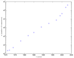
The figure shows the number of transistors in 13 microprocessors as a function of the year of their introduction. The plot suggests that we can obtain a good fit with a function of the form $n(t)=\alpha^{t-t_0}$ , where $t$ is the year, $n(t)$ is the number of transistors at year $t$ , and $\quad \alpha>0$ and $t_0$ are model parameters. This model results in a straight line if we plot $n(t)$ on a logarithmic scale versus $t$ on a linear scale, as is done in the figure.

1. Moore’s law describes a long-term trend in the history of computing hardware and states that the number of transistors that can be placed inexpensively on an integrated circuit has doubled approximately every two years. In this problem, we investigate the validity of the claim via least-squares.

Using the problem data below:

show how to estimate the parameters $\alpha, t_0$ using least-squares, that is, via a problem of the form

$\min _x\|A x-y\|_2$

Make sure to define precisely the data $A,y$ and how the variable $x$ relates to the original problem parameters $\alpha, t_0$ . (Use the notations $n = \begin{pmatrix} n_1 \\ \ldots \\ n_{13}\end{pmatrix} \in \mathbb{R}^{13}$ for the number of processors, and $t = \begin{pmatrix} t_1 \\ \ldots \\ t_{13}\end{pmatrix} \in \mathbb{R}^{13}$ for the corresponding years. You can assume that no component of $x$ is zero at optimum.)

a. Is the solution to the problem above unique? Justify carefully your answer, and give the expression for the unique solution $x^*$ in terms of $A,y$ .

b. The solution to the problem yields $\alpha=1.4257, t_0=1949.7$ . Is this estimate consistent with the so-called Moore’s law, which states that the number of transistors per integrated circuit roughly doubles every two years?

2. The Michaelis–Menten model for enzyme kinetics relates the rate $y$ of an enzymatic reaction, to the concentration $x$ of a substrate, as follows:

$y=\frac{\beta_1 x}{\beta_2+x}$

where $\beta_i, i=1,2$ , are parameters.

a. Show that the model can be expressed as a linear relation between the values $1 / y$ and $1 / x$ .

b. Use this expression to fit the parameter $\beta$ using linear least-squares.

c. The above approach has been found to be quite sensitive to errors in input data. Can you experimentally confirm this opinion?

Hint: generate noisy data from parameter values $\beta_1=3.4$ and $\beta_2=0.4$ .

License

Icon for the Creative Commons Attribution-NonCommercial-NoDerivatives 4.0 International License

27.1. Standard forms

27.2. Applications

License

Share This Book