HYPERPLANES AND HALF-SPACES

Alicia Y. Tsai; Authors: Laurent EI Ghaoui; Contributors: Phan Hoang, Tony Tin, Ha To Tam, Nguyen Van Kep, Le Dinh Nam, Juliette Decugis, Nguyen Quoc Cuong.; Giuseppe C. Calafiore

5 HYPERPLANES AND HALF-SPACES

5.1. Hyperplanes

A hyperplane is a set described by a single scalar product equality. Precisely, a hyperplane in $\mathbb{R}^n$ is a set of the form

$\begin{align*} \mathbf{H} = \{x: a^Tx = b\}, \end{align*}$

where $a \in \mathbb{R}^n$ , $a \neq 0$ , and $b \in \mathbb{R}$ are given. When $b=0$ , the hyperplane is simply the set of points that are orthogonal to $a$ ; when $b \neq 0$ , the hyperplane is a translation, along direction $a$ , of that set.

If $x_0 \in {\bf H}$ , then for any other element $x \in {\bf H}$ , we have

$\begin{align*} b = a^Tx_0 = a^Tx. \end{align*}$

Hence, the hyperplane can be characterized as the set of vectors $x$ such that $x - x_0$ is orthogonal to $a$ :

$\begin{align*} \mathbf{H} = \{x: a^T(x-x_0) = 0\}. \end{align*}$

Hyperplanes are affine sets, of dimension $n-1$ (see the proof here). Thus, they generalize the usual notion of a plane in $\mathbb{R}^3$ . Hyperplanes are very useful because they allows to separate the whole space in two regions. The notion of half-space formalizes this.

Example 1: A hyperplane in $\mathbb{R}^3$ .

Consider an affine set of dimension $2$ in $\mathbb{R}^3$ , which we describe as the set of points $x$ in $\mathbb{R}^3$ such that there exists two parameters $\lambda_1, \lambda_2$ such that
$x = \begin{pmatrix} 3\lambda_1-4\lambda_2 + 4 \\ \lambda_1 \\ \lambda_2 \end{pmatrix} = \begin{pmatrix} 4 \\ 0 \\ 0 \end{pmatrix} + \lambda_1 \begin{pmatrix} 3 \\ 1 \\ 0 \end{pmatrix} + \lambda_2 \begin{pmatrix} -4 \\ 0 \\ 1 \end{pmatrix}.$
The set $\mathbf{H}$ can be represented as a translation of a linear subspace: $\mathbf{H} = x_0 + \mathbf{L}$ , with
$x_0 := \begin{pmatrix} 4 \\ 0 \\ 0 \end{pmatrix},$
and $\mathbf{L}$ the span of the two independent vectors
$u := \begin{pmatrix} 3 \\ 1 \\ 0 \end{pmatrix}, \quad v := \begin{pmatrix} -4 \\ 0 \\ 1 \end{pmatrix}.$
Thus, the set $\mathbf{H}$ is of dimension $2$ in $\mathbb{R}^3$ , hence it is a hyperplane. In $\mathbb{R}^3$ , hyperplanes are ordinary planes. We can find a representation of the hyperplane in the standard form
$\mathbf{H} = \left\{ x \,:\, a^T(x-x_0) = 0 \right\}.$
We simply find $a$ that is orthogonal to both $u$ and $v$ . That is, we solve the equations
$0 = a^T u = 3a_1 + a_2, \quad 0 = a^T v = -4a_1 + a_3.$
The above leads to $a = (a_1, -3a_1, 4a_1)$ . Choosing for example $a_1 = 1$ leads to $a=(1,-3,4)$ .
		The hyperplane $\mathbf{H}$ can be expressed as $x_0 + \mathbf{span}(u, v)$ , where $x_0$ is a particular element, and $u, v$ are two independent vectors. The set $\mathbf{H}$ is represented in light blue; it is a translation of the corresponding span $\mathbf{L} = \mathbf{span}(u, v)$ . Any point $x$ in $\mathbf{H}$ is such that $x - x_0$ belongs to $\mathbf{L}$ . Thus, we can represent the hyperplane as the set of points such that $x - x_0$ is orthogonal to $a$ , where $a$ is any vector orthogonal to both $u, v$ .

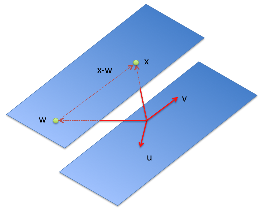
5.2. Projection on a hyperplane

Consider the hyperplane ${\bf H} = \{x: a^Tx = b\}$ , and assume without loss of generality that $a$ is normalized ( $||a||_2 =1$ ). We can represent ${\bf H}$ as the set of points $x$ such that $x- x_0$ is orthogonal to $a$ , where $x_0$ is any vector in ${\bf H}$ , that is, such that $a^Tx_0 = b$ . One such vector is $x_{proj}:= ba$ .

By construction, $x_{proj}$ is the projection of $0$ on ${\bf H}$ . That is, it is the point on ${\bf H}$ closest to the origin, as it solves the projection problem

$\begin{align*} \min\limits_x ||x||_2: x \in \mathbf{H} \end{align*}$

Indeed, for any $x \in {\bf H}$ , using the Cauchy-Schwartz inequality:

$\begin{align*} ||x_0||_2 = |b| = |a^Tx| \leq ||a||_2 \cdot ||x||_2 = ||x||_2, \end{align*}$

and the minimum length | $b$ | is attained with $x_{proj} = ba$ .

5.3. Geometry of hyperplanes

	Geometrically, a hyperplane ${\bf H} = \{x: a^Tx = b\}$ , with $\|\|a\|\|_2 = 1$ , is a translation of the set of vectors orthogonal to $a$ . The direction of the translation is determined by $a$ , and the amount by $b$ .
	Precisely, \| $b$ \| is the length of the closest point $x_0$ on ${\bf H}$ from the origin, and the sign of $b$ determines if ${\bf H}$ is away from the origin along the direction $a$ or $-a$ . As we increase the magnitude of $b$ , the hyperplane is shifting further away along $\pm a$ , depending on the sign of $b$ .
	In a 3D space, a hyperplane corresponds to a plane. In the image on the left, the scalar $b$ is positive, as $x_0$ and $a$ point to the same direction.

5.4. Half-spaces

A half-space is a subset of $\mathbb{R}^n$ defined by a single inequality involving a scalar product. Precisely, a half-space in $\mathbb{R}^n$ is a set of the form

$\begin{align*} \mathbf{H} = \{x: a^Tx \ge b\}, \end{align*}$

where $a \in \mathbb{R}^n$ , $a \neq 0$ , and $b \in \mathbb{R}$ are given.

Geometrically, the half-space above is the set of points such that ${a^T(x-x_0) \ge 0$ , that is, the angle between $x - x_0$ and $a$ is acute (in $[-90^{\circ}; +90^{\circ}]$ ). Here $x_0$ is the point closest to the origin on the hyperplane defined by the equality $a^Tx = b$ . (When $a$ is normalized, as in the picture, $x_0 = ba$ .)


	The half-space $\{x: a^Tx \ge b\},$ is the set of points such that $x-x_0$ forms an acute angle with $a$ , where $x_0$ is the projection of the origin on the boundary of the half-space.
	The image on the left is a visualization of half-spaces in a 3D context.

License

Icon for the Creative Commons Attribution-NonCommercial-NoDerivatives 4.0 International License

5.1. Hyperplanes

5.2. Projection on a hyperplane

5.3. Geometry of hyperplanes

5.4. Half-spaces

License

Share This Book