Image compression
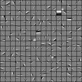
To represent the image in terms of the dictionary, we would like to find coefficients ![]() ,
, ![]() such that
such that
![Rendered by QuickLaTeX.com \[y = \sum_{j=1}^{n} x_j a_j,\]](https://pressbooks.pub/app/uploads/quicklatex/quicklatex.com-c83c7fa0d774056fefc20e5431c7ebfe_l3.png)
or, more compactly, ![]() .
.
If the representation of the image (that is, the vector ![]() ) has many zeros (we say:
) has many zeros (we say: ![]() is sparse), then we can represent the entire image with only a few values (the components of
is sparse), then we can represent the entire image with only a few values (the components of ![]() that are not zero). We may then, for example, send the image over a communication network at high speed. Provided the receiver has the dictionary handy, it can reconstruct perfectly the image.
that are not zero). We may then, for example, send the image over a communication network at high speed. Provided the receiver has the dictionary handy, it can reconstruct perfectly the image.
In practice, it may be desirable to trade off the sparsity of the representation (via ![]() ) against the accuracy of the representation. Namely, we may prefer a representation
) against the accuracy of the representation. Namely, we may prefer a representation ![]() that achieves
that achieves ![]() only approximately but has way more zeros. The process of searching for a good sparsity/accuracy trade-off is called image compression.
only approximately but has way more zeros. The process of searching for a good sparsity/accuracy trade-off is called image compression.

