PRINCIPAL COMPONENT ANALYSIS

Alicia Y. Tsai; Authors: Laurent EI Ghaoui; Contributors: Phan Hoang, Tony Tin, Ha To Tam, Nguyen Van Kep, Le Dinh Nam, Juliette Decugis, Nguyen Quoc Cuong.; Giuseppe C. Calafiore

31 PRINCIPAL COMPONENT ANALYSIS

31.1. Projection on a line via variance maximization

Consider a data set of $n$ points $x_j$ , $j = 1, \cdots, n$ in $\mathbb{R}^m$ . We can represent this data set as a $m \times n$ matrix $X = [x_1, \cdots, x_n]$ , where each $x_j$ is a $n$ -vector. The goal of the variance maximization problem is to find a direction $u \in \mathbb{R}^m$ such that the sample variance of the corresponding vector $u^TX = (u^Tx_1, \cdots, u^Tx_n)$ is maximal.

Recall that when $u$ is normalized, the scalar $u^Tx$ is the component of $x$ along $u$ , that is, it corresponds to the projection of $x$ on the line passing through $0$ and with direction $u$ .

Here, we seek a (normalized) direction $u$ such that the empirical variance of the projected values $u^Tx_j$ , $j = 1, \cdots, n$ , is large. If $\hat{x}$ is the vector of averages of the $x_j$ ‘s, then the average of the projected values is $u^T\hat{x}$ . Thus, the direction of maximal variance is one that solves the optimization problem

$\begin{align*} \max\limits_{u: ||u||_2=1} \frac{1}{n} \sum\limits_{j=1}^n \left((x_j-\hat{x})^Tu\right)^2. \end{align*}$

The above problem can be formulated as

$\begin{align*} \max\limits_{u: ||u||_2=1} u^T {\textstyle \Sigma} u, \end{align*}$

where

$\begin{align*} {\textstyle \Sigma} := \frac{1}{n}\sum\limits_{j=1}^n (x_j - \hat{x}) (x_j-\hat{x})^T \end{align*}$

is the $m \times m$ sample covariance matrix of the data.

We have seen the above problem before, under the name of the Rayleigh quotient of a symmetric matrix. Solving the problem entails simply finding an eigenvector of the covariance matrix $\sum$ that corresponds to the largest eigenvalue.

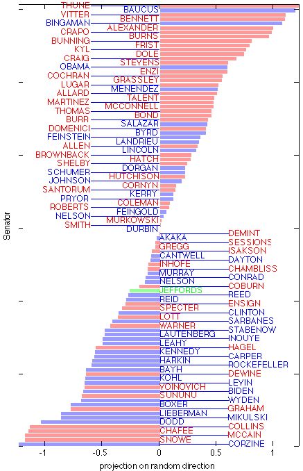
Maximal variance direction for the Senate voting data. This image shows the scores assigned to each Senator along the direction of maximal variance, $u^T_{\max}(x_j-\hat{x})$ , $j = 1, \cdots, n$ , with $u_{\max}$ a normalized eigenvector corresponding to the largest eigenvalue of the covariance matrix $\sum$ . Republican Senators tend to score negatively, while we find many Democrats on the positive score (obviously the signs themselves don’t count here, as we could switch $u$ to $-u$ ; only the order is important). Hence the direction could be interpreted as revealing the party affiliation. The two Senators that are in the opposite group (especially Sen. Chaffee) have indeed sometimes voted against their party.

Note that the largest absolute score obtained in this plot is about 18 times bigger than that observed on the projection in a random direction. This is consistent with the fact that the current direction has a maximal variance.

31.2. Principal component analysis

Main idea

The main idea behind principal component analysis is to first find a direction that corresponds to maximal variance between the data points. The data is then projected on the hyperplane orthogonal to that direction. We obtain a new data set and find a new direction of maximal variance. We may stop the process when we have collected enough directions (say, three if we want to visualize the data in 3D).

It turns out that the directions found in this way are precisely the eigenvectors of the data’s covariance matrix. The term principal components refers to the directions given by these eigenvectors. Mathematically, the process thus amounts to finding the eigenvalue decomposition of a positive semi-definite matrix, the covariance matrix of the data points.

Projection on a plane

The projection used to obtain, say, a two-dimensional view with the largest variance, is of the form $x \rightarrow Px$ , where $P=[u_1, u_2]^T$ is a matrix that contains the eigenvectors corresponding to the first two eigenvalues.

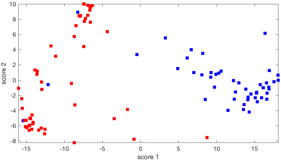Two-dimensional projection of the Senate voting matrix: This particular planar projection uses the two eigenvectors corresponding to the largest two eigenvalues of the data’s covariance matrix. It seems to allow to cluster of the Senators along party lines and is therefore more informative than, say, the plane corresponding to the two smallest eigenvalues.

31.3. Explained variance

The total variance in the data is defined as the sum of the variances of the individual components. This quantity is simply the trace of the covariance matrix since the diagonal elements of the latter contain the variances. If $\Sigma$ has the EVD $\Sigma = U \Lambda U^T$ , where $\Lambda = {\bf diag}(\lambda_1, \cdots, \lambda_n)$ contains the eigenvalues, and $U$ an orthogonal matrix of eigenvectors, then to total variance can be expressed as the sum of all the eigenvalues:

$\begin{align*} {\bf Tr} \Sigma = {\bf Tr}(U\Lambda U^T) = {\bf Tr} (U^TU\Lambda) = {\bf Tr} \Lambda = \lambda_1 + \cdots + \lambda_n. \end{align*}$

When we project the data on a two-dimensional plane corresponding to the eigenvectors $u_1, u_2$ associated with the two largest eigenvalues $\lambda_1, \lambda_2$ , we get a new covariance matrix $P \Sigma P^T$ , where $P = [u_1, u_2]^T$ the total variance of the projected data is

$\begin{align*} {\bf Tr}(P\Sigma P^T) = \lambda_1 + \lambda_2. \end{align*}$

Hence, we can define the ratio of variance ‘‘explained’’ by the projected data as the ratio:

$\begin{align*} \frac{\lambda_1 + \lambda_2}{\lambda_1 + \cdots + \lambda_n}. \end{align*}$

If the ratio is high, we can say that much of the variation in the data can be observed on the projected plane.

This image shows the eigenvalues of the $m \times m$ covariance matrix of the Senate voting data, which contains the covariances between the votes of each pair of Senators. Clearly, the eigenvalues decrease very fast. One is tempted to say that In this case, the ratio of explained to total variance is almost $90%$ , which indicates that ‘‘most of the information’’ is contained in the first eigenvalue. Since the corresponding eigenvector almost corresponds to a perfect ‘‘party line’’, we can say that party affiliation explains most of the variance in the Senate voting data.

License

Icon for the Creative Commons Attribution-NonCommercial-NoDerivatives 4.0 International License