8.3 Economic Order Quantity (EOQ)
The Economic Order Quantity (EOQ) is a foundational concept in inventory management. It provides a model to determine the optimal order quantity a firm should maintain to minimize the total inventory costs. At its core, the EOQ model is designed to strike a balance between the costs associated with holding inventory and the costs related to ordering inventory.
It’s important to note that the basic EOQ model focuses primarily on these two costs and does not factor in other potential costs like stockouts, obsolescence, or lost goodwill. This makes the model a simplified representation, but it’s still a valuable tool for many businesses, especially when used as a starting point for more complex inventory decisions.
Assumptions of the EOQ Model:
- Constant Demand: The model assumes that the demand for the product is known and remains consistent throughout the period.
- Instantaneous Replenishment: Once an order is placed, the inventory is replenished immediately, meaning there’s no lead time.
- Only Ordering and Holding Costs: The model considers only the costs of ordering and holding inventory. Other costs, like stockouts or obsolescence, are not factored in.
- Fixed Order Cost: The cost of placing an order remains constant, regardless of the order size.
- Fixed Holding Cost: The cost to hold or store an item in inventory for a specific period remains constant.
- No Quantity Discounts: The purchase price of the product is constant, meaning no discounts are given for bulk purchases.
- No Stockouts: The model operates under the assumption that stockouts are not allowed or are not a consideration.
While the EOQ model is based on these assumptions, it’s essential to recognize that real-world scenarios might not always align perfectly. However, the model provides a foundational understanding and a starting point for businesses to delve deeper into their specific inventory challenges and refine their strategies accordingly.
8.3.1 Understanding the EOQ Model
Let us delve into the Economic Order Quantity (EOQ) model using a practical example to better grasp its concepts. Consider a firm that has a yearly demand for 80,000 widgets. They’ve calculated their holding cost (Ch) to be $1 per item per year and their ordering cost (Co) to be $400 per order. Now, suppose the firm decides to order 20,000 units at one time.
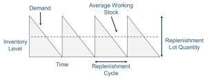
In this scenario, the firm will commence with an inventory of 20,000 units. Given the constant demand, the inventory will deplete to zero at a steady rate. As soon as the inventory reaches zero, it is instantaneously replenished, bringing the stock back up to 20,000 units. This cycle of depleting and replenishing will continue throughout the year. Since the annual demand is 80,000 units and each order brings in 20,000 units, this cycle will repeat itself precisely four times in the year. The inventory position over the year is depicted in the sawtooth diagram shown below.
Ordering Cost Calculation:
Yearly Demand (D): 80,000 units
Size of one order (Q): 20,000 units
Ordering cost per order (Co): $400
Given the above, the number of orders the firm will place in a year is calculated as: Number of Orders (N)= D/Q = 80,000/20,000 = 4 orders per year
The total ordering cost for the year is then:
Total Ordering Cost (T0) = N × Ordering cost per order
Total Ordering Cost= 4 * $400 = $1,600
Holding Cost Calculation:
The holding cost (Ch) is provided as $1 per item per year. If a firm were to maintain a constant inventory of 20 units throughout the year, the total holding cost would amount to 20 * $1 = $20. However, as indicated in the diagram above, the firm’s inventory isn’t constant. It peaks at 20,000 units and drops to zero. To account for this fluctuation, we need to calculate the average inventory in the cycle:
Average Inventory: Iavg = [latex]\frac{(Imax + Imin)}{ 2}[/latex]
Where Imax represents the maximum inventory and Imin is the minimum inventory value in the cycle.
In this scenario: Iavg = [latex]\frac{(20,000 + 0)}{ 2}[/latex] = 10,000 units.
Total Holding Cost, Th = Average Inventory × Holding Cost per Unit
Th = 10,000 * $1 = $10,000.
Consequently, the total inventory-related costs is the sum of ordering and holding costs:
T = To+ Th
T = $1,600 + $10,000 = $11,600.
If the firm decides to have an order size is 5000, the total costs would be different:
Average Inventory, Iavg = [latex]\frac{(5000 + 0)}{ 2}[/latex] = 2,500 units.
Total Holding Cost, Th = Average Inventory × Holding Cost per Unit
Th = 2,500 * $1 = $2,500.
Given the yearly demand of 80,000 units and an order size of 5,000 units, the firm will place 16 orders throughout the year.
Total Ordering Cost, To = Number of Orders × Cost per Order
To = 16 * $400 = $6,400.
Total inventory-related costs,
T = To+Th
T = $6,400 + $2,500 = $8,900.
We can represent both these cases in this table:
| Order Size (units) | Total Holding Cost (Th) | Total Ordering Cost (To) | Total Cost (T) |
| 20,000 | $10,000 | $1,600 | $11,600 |
| 5,000 | $2,500 | $6,400 | $8,900 |
From the table, we can observe the following:
- As the order size increases, the Total Holding Cost (Th) also increases. This is because a larger order size means more inventory is held on average throughout the year, leading to higher holding costs.
- Conversely, as the order size increases, the Total Ordering Cost (To) decreases. A larger order size means fewer orders are placed throughout the year, resulting in lower ordering costs.
So, one way to find the lowest inventory cost is to calculate the total cost (T) for multiple order sizes and find the order size at which the total cost is minimum. This is presented in the table below:
| Order Size (units) | Total Holding Cost (Th) | Total Ordering Cost (To) | Total Cost (T) |
| 2,500 | $1,250 | $ 12,800 | $14,050 |
| 5,000 | $2,500 | $ 6,400 | $8,900 |
| 6,000 | $3,000 | $ 5,333 | $8,333 |
| 7,000 | $3,500 | $ 4,571 | $8,071 |
| 8,000 | $4,000 | $ 4,000 | $8,000 |
| 10,000 | $5,000 | $ 3,200 | $8,200 |
| 12,000 | $6,000 | $ 2,667 | $8,667 |
| 15,000 | $7,500 | $ 2,133 | $9,633 |
| 20,000 | $10,000 | $ 1,600 | $11,600 |
We can represent the table in this chart:
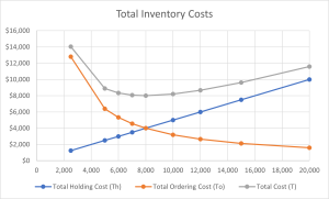
As we can see, the lowest total cost is for an order size of 8000 units when the total holding costs (Th) is equal to the total ordering costs (To). This order size for the lowest total inventory related costs is called the Economic Order Quantity (EOQ).
From the graph, it will be evident that as the order size increases, the total cost first decreases, reaches a minimum, and then starts to increase again. This U-shaped curve is characteristic of the EOQ model. The point at which the total cost is minimized, in this case at an order size of 8,000 units, is the optimal order quantity. This is the quantity that minimizes the combined holding and ordering costs, ensuring the most cost-effective inventory management for the firm.
Building on our previous discussion, while the tabular method provides clarity on how costs change with order size, it’s not the most efficient way to determine the optimal order quantity in real-world scenarios. Especially for businesses dealing with a multitude of products, manually calculating costs for various order sizes would be cumbersome. Fortunately, there’s a more streamlined approach to find the Economic Order Quantity (EOQ) that minimizes the total inventory-related costs. The minimum cost, representing a balance between holding and ordering costs, is expressed as:
Total Holding Cost (Th) = Total Ordering Cost (To)
[latex]\frac{D}{Q}\ \ast\ C_0=\ \frac{D}{2}\ \ast\ C_h[/latex]
Therefore, extracting Q out of the equation we have: the EOQ formula.
[latex]\ Q\ =\ EOQ\\ =\ \sqrt{\frac{2\ *\ D\ *\ C_o}{C_h}}[/latex]
Where:
- EOQ = Economic Order Quantity (the optimal order size)
- D = Annual demand or usage for the inventory item
- Co = Cost to place a single order (ordering cost)
- Ch = Cost to hold one unit of inventory for one year (holding or carrying cost)
The EOQ formula is derived from the principle of balancing the ordering and holding costs, ensuring that the sum of these costs is minimized. By using this formula, businesses can quickly determine the optimal order size that minimizes total inventory costs.
Applying the formula to our example:
Given:
D = 80,000 units (annual demand)
Co = $400 (ordering cost per order)
Ch = $1 (holding cost per unit per year)
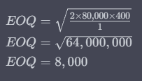
Thus, using the EOQ formula, the optimal order size that minimizes the total inventory-related costs for the firm is 8,000 units. This result aligns with our earlier tabular method, validating the efficiency and accuracy of the EOQ formula.
