9.4 Quantitative Methods
At the heart of quantitative forecasting lies a fundamental assumption: the patterns observed in historical data will, to some extent, repeat in the future. To illustrate, consider the sales of winter coats. While the exact number of coats sold each winter may vary, the general pattern of increased sales during colder months and decreased sales during warmer months is likely to persist year after year. Similarly, a theme park might observe higher visitor numbers during school holidays compared to school terms. This doesn’t imply that the exact number of visitors will be the same every holiday, but the trend of increased visitors during holidays is expected to continue. This foundational principle doesn’t suggest that the future will mirror the past exactly. Instead, it posits that the variability and inherent patterns seen in historical data will be reflected in future forecasts.
Time Series Analysis: This technique revolves around dissecting historical data to discern discernible patterns and trends. Once identified, these patterns can be extrapolated to predict future values. For instance, a retailer might analyze monthly sales data over several years to identify seasonal peaks and troughs. By recognizing these recurring patterns, the retailer can better anticipate sales for the upcoming months. While this chapter will introduce a few basic time series methods, it’s worth noting that the realm of time series analysis is vast and continually evolving.
Causal Modeling: Rather than solely relying on past data of the variable being forecasted, causal modeling seeks to understand the relationships between that variable and other influencing factors. For example, a car manufacturer might develop a model that considers factors like GDP growth, fuel prices, and interest rates to forecast car sales. By simulating how changes in these factors might impact sales, the manufacturer can make more informed production and marketing decisions.
Machine Learning: Emerging from the expansive field of computer science, machine learning focuses on crafting algorithms that can learn from and make predictions based on data. These algorithms, once trained on historical data, can forecast a myriad of variables. A tech company, for instance, might employ machine learning to predict user engagement based on past user behavior, platform changes, and external events. Such forecasts can guide feature development, marketing strategies, and user support initiatives.
Each of these method classes offers unique advantages and is suited for specific scenarios. By understanding their underlying principles and applications, businesses can select the most appropriate technique for their forecasting needs, ensuring more accurate and actionable predictions.
9.4.1 Time Series Methods
Time series methods are a cornerstone of quantitative forecasting, particularly favored for their applicability in medium-term and short-term predictions. At their core, these methods revolve around the analysis of data points collected or recorded at specific time intervals. Whether it’s a retailer predicting monthly sales or a utility company forecasting daily electricity consumption, time series methods offer a structured approach to understanding past patterns and predicting future value
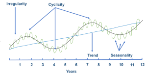
A key strength of time series analysis is its ability to decompose demand data into distinct components, each representing different patterns or influences on the data:
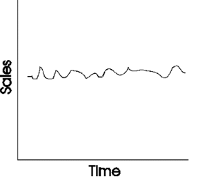
Level: This represents the average value in the series. For instance, if we’re looking at monthly sales of a product, the level would be the average monthly sales over a given period.
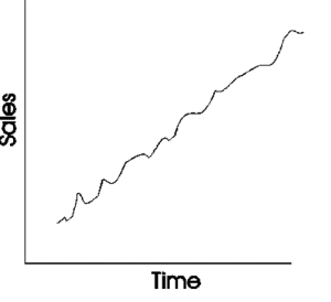
 Trend: This captures any consistent upward or downward movement in the data over time. For a burgeoning product, this might represent a steady increase in sales month over month. Alternatively, a product nearing the end of its life cycle might exhibit a consistent downward trend.
 Season: Seasonal components capture regular patterns that repeat over specific intervals. A retailer might observe higher sales every weekend, indicating a weekly seasonal pattern. Ice cream sales might show a seasonal spike every summer, representing an annual seasonality. Electricity utilities might notice a peak in consumption around 2 pm every day, pointing to a daily seasonal pattern.

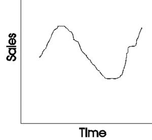
Cycle: Cycles are long-term patterns driven by economic or other broad factors. They don’t have a fixed repetition like seasons but show up as extended periods of rises and falls. For instance, the real estate market might go through cycles of boom and bust over decades, influenced by broader economic conditions.
Time series methods work by first decomposing historical demand into these components. Each component is then forecasted independently, leveraging the inherent patterns and characteristics it exhibits. Once individual forecasts for the level, trend, season, and cycle are generated, they are combined to produce the final forecast.
 A few prominent time series methods include:
The Naive Forecast Method: The simplest and most straightforward methods for making predictions or forecasts. This method is often used as a baseline or reference point in forecasting to evaluate the performance of more complex forecasting models.
The Naive Forecast Method involves making a forecast for a future period based solely on the observed value of the most recent period. In other words, it assumes that future values will be the same as the most recent historical value. Mathematically, the Naive Forecast is represented as:
Naive Forecast for period t+1=Value observed in period t
Example, if the observed sales value (actual) for January is 120 units, then the forecast for February is 120 units.
Moving Averages: This method calculates the average of a set number of past periods to produce the forecast for the next period. It’s especially useful for data with no clear trend or seasonal pattern.
Exponential Smoothing: This technique gives different weights to past observations, with more recent data typically receiving more weight. It’s adaptable and can handle data with trends and seasonality.
ARIMA (AutoRegressive Integrated Moving Average): A more advanced method, ARIMA models the relationships between an observation and a number of lagged observations.
Each of these methods offers unique advantages and is suited for specific scenarios. The choice of method often hinges on the nature of the data, the forecasting horizon, and the specific challenges posed by the demand pattern.
In the subsequent section, we will delve deeper into two of these methods, specifically focusing on simple moving averages and exponential smoothing, to provide a more detailed understanding of their applications and nuances.
9.4.1.1 Simple Moving Average
The Simple Moving Average (SMA) is a straightforward yet effective time series forecasting method. At its core, the SMA for a given period is calculated by taking the average of the previous ‘n’ periods. This approach ensures that fluctuations in individual periods are smoothed out, providing a clearer view of underlying trends.
For instance:
- 3-Month Moving Average: If a retailer recorded sales of 100, 110, and 90 units for January, February, and March respectively, the 3-month moving average forecast for April would be the average of these three months:
[latex]\frac{(100 + 110 + 90)}{ 3} = 100 units[/latex] - 4-Month Moving Average: Using the same example, if we also had a sales figure of 105 units for April, the 4-month moving average forecast for May would be:
[latex]\frac{(100 + 110 + 90 + 105)}{ 4} = 101.25 units[/latex] - 5-Month Moving Average: If May had sales of 95 units, then the 5-month moving average forecast for June would be:
[latex]\frac{(100 + 110 + 90 + 105 + 95)}{ 5} = 100 units[/latex]
One of the key considerations when using the SMA method is selecting the appropriate length for the moving average. A longer period, such as a 12-month moving average, will produce a smoother forecast, less sensitive to short-term fluctuations or extreme demand values. This can be particularly beneficial when trying to identify longer-term trends or when the data has occasional outliers. However, it’s essential to note that while longer moving averages provide stability, they might be slower to respond to genuine shifts in demand patterns.
In essence, the Simple Moving Average method offers a balance between capturing the inherent variability in data and providing stable forecasts, making it a versatile tool in a forecaster’s toolkit.
9.4.1.2 Simple Exponential Smoothing
Simple Exponential Smoothing (SES) is a favored method for time series forecasting, especially when data exhibits no clear trend or seasonality. The essence of SES is to assign exponentially decreasing weights to past observations, ensuring that more recent data points have a more significant influence on the forecast, while older data points have a diminishing impact.
The formula for Simple Exponential Smoothing is given by:
Ft+1 = α × Dt + (1−α) × Ft
Where:
- Ft+1 is the forecast for the next period.
- Dt is the actual demand in the current period.
- Ft is the forecast for the current period.
- α is the smoothing factor, a value between 0 and 1.
Example 1:
Suppose a product had a forecasted demand of 100 units for January (Ft). The actual demand for January (Dt) turned out to be 110 units. Using a smoothing factor α of 0.2, the forecast for February (Ft+1) would be:
Ft+1 = 0.2 × 110 + (1−0.2) × 100
Ft+1 = 22 + 80 = 102
So, the forecast for February would be 102 units.
Example 2:
Continuing from the previous example, let’s say the actual demand for February was 105 units. To forecast the demand for March using the same smoothing factor:
Ft+1 = 0.2×10⁵ + (1−0.2)×102
Ft+1 = 21 + 81.6 = 102.6
Thus, the forecast for March would be approximately 102.6 units.
The key parameter in SES is the smoothing factor, often denoted as α (alpha). This factor determines the sensitivity of the forecast to changes in historical demand:
- When α is 0, the forecast becomes entirely insensitive to historical demand variations. In essence, it becomes a flat line, only considering the initial forecast and ignoring all subsequent data.
- Conversely, when α is 1, the forecast becomes extremely sensitive, relying solely on the most recent demand observation. The forecast will adjust immediately to the last observed value, making it highly reactive to any changes.
For a practical understanding, consider a scenario where a product’s demand has been relatively stable but recently started to increase. A higher alpha would quickly adjust the forecast upwards to match this new trend, while a lower alpha would be slower to recognize and adapt to this change.
Selecting the right value for α is crucial. A value too close to 0 might make the forecast too sluggish to adapt to genuine changes in demand, while a value too close to 1 might make it overly reactive to random fluctuations, potentially leading to overcorrections.
In summary, Simple Exponential Smoothing offers a dynamic approach to forecasting, allowing forecasters to control the sensitivity of their predictions to historical data. By tuning the smoothing factor, forecasters can strike a balance between stability and reactivity, ensuring that their forecasts are both accurate and robust.
