8.4 Systems of How Much to Order and When to Order
8.4.1 How Much to Order
Building on our exploration of the EOQ model, it’s evident that while EOQ provides a mathematical approach to determine the optimal order quantity, it’s just one of the many methods available. The EOQ model, despite its utility, has certain concerns:
- Assumptions: The EOQ model operates under several assumptions, such as constant demand and instantaneous replenishment, which might not hold true for all businesses.
- Static Nature: The model doesn’t account for dynamic changes in market conditions, demand fluctuations, or supply chain disruptions.
- Exclusion of Other Costs: While the model considers ordering and holding costs, it often overlooks other significant costs like stockouts, obsolescence, or lost goodwill.
- Lack of Flexibility: The EOQ model might not be adaptable to businesses with diverse product lines, varying demand patterns, or those operating in volatile markets.
Given these concerns, the EOQ model might not always be the most practical choice for firms. Therefore, businesses often explore other systems to decide how much to order. Broadly, there are two primary options:
a. Lot-for-Lot Systems:
In a lot-for-lot system, the order quantity matches the exact demand for a specific period. This approach minimizes holding costs since there’s no excess inventory. It’s particularly suitable for products with irregular demand patterns or those with a short shelf life. Firms following Just-In-Time (JIT) inventory systems often adopt the lot-for-lot approach. JIT emphasizes reducing waste by ordering and producing only what is needed, when it’s needed. We’ll delve deeper into the intricacies of JIT in a subsequent chapter.
b. Lot Size-Based Ordering:
In this system, preference is given to ordering in specific lot sizes, often influenced by external factors. For instance:
- Full Load Preference: Companies might prefer to order in full truckloads or container loads to optimize transportation costs.
- Discounts: Ordering in select lot sizes might make a firm eligible for bulk purchase discounts, leading to reduced per-unit costs.
- EOQ: As we’ve seen, EOQ is a lot size-based ordering system where the order quantity is determined based on minimizing associated costs.
In conclusion, while the EOQ model offers a structured approach to determine order quantities, it’s essential for businesses to evaluate its applicability in their specific context and consider alternative systems that might be more aligned with their operational realities and strategic goals.
8.4.2 When to Order: Key Systems
Determining the optimal quantity to order is only half the battle in inventory management. The other crucial aspect is deciding when to place that order. Two primary systems guide this decision-making process: (1) Reorder Point (ROP) based ordering and (2) Periodic ordering.
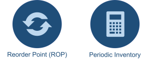
Reorder Point (ROP) Based Ordering:
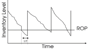
The Reorder Point (ROP) is the inventory level at which a new order should be placed to replenish stock before it runs out. The primary factor influencing ROP is the lead time, which is the duration between placing an order and receiving the inventory.
Example: Let’s consider a firm that uses 20 units of a particular item every day. If the lead time for replenishing this item is 4 days, then the firm would need 80 units (20 units/day x 4 days) to cover its needs during this period. Thus, the reorder point would be set at 80 units. This means that as soon as the inventory level drops to 80 units, a new order should be placed to ensure continuous availability.
ROP = (Demand per period) * (number of periods in the LT)
Another Example: Suppose:
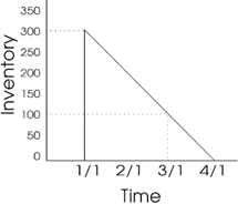
D = 1200 units per year (100 units per month)
Q = 300 units
Lead Time = LT = 1 month.
When should we place the order?
However, the above calculation assumes a constant and predictable demand. In reality, demand can fluctuate due to various factors, from seasonal variations to sudden market changes. To account for these uncertainties, businesses often maintain a safety stock. The revised ROP formula, considering safety stock, is:
ROP=(Demand during Lead Time)+Safety Stock
ROP=DLT+SS
Where:
- DLT is the demand during lead time = Average Demand per period * number of periods in LT
- SS is the safety stock = Z × σ × √LT
Safety stock acts as a buffer against uncertainties in demand or supply. It ensures that even if there’s an unexpected spike in demand or a delay in replenishment, the business can continue to meet customer requirements without any interruptions.
Safety stock can manifest in various forms across the supply chain. For instance, a company might maintain additional raw material inventory to buffer against erratic suppliers or extended delivery lead times. Work-In-Progress (WIP) buffers might be in place to handle unscheduled maintenance breakdowns in machinery. Similarly, there might be Maintenance, Repair, and Operations (MRO) buffers. Regardless of its form, the underlying principle of safety stock remains consistent: it’s a trade-off between the benefits of having extra inventory (like ensuring customer satisfaction or production continuity) and the associated costs (like holding costs).
While the concept of safety stock is straightforward, determining the right amount to hold can be complex. Too little safety stock can lead to stockouts and lost sales, while too much can inflate inventory holding costs. Hence, businesses need a systematic approach to set safety stock levels.
Calculating Safety Stock using the Normal Distribution
One widely accepted method to calculate safety stock is based on the normal distribution of demand or lead time variability. The normal distribution, often referred to as the bell curve, describes how values of a variable are distributed in a dataset. Most values cluster around the central mean (or average), and fewer and fewer are found as you move away from the mean in either direction.
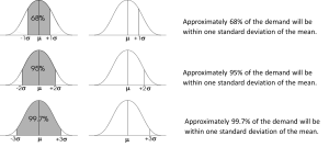 Knowing these facts enables us to easily determine the chances (probabilities) of demand occurring more than or less than or between any of the values. For example, if µ=100, σ = 20, the probability that the demand will exceed 140 is 2.5% (from the second set of the above figures).
Given the assumption of normally distributed demand, the safety stock can be calculated using the formula:
Safety Stock = Z × σ × √LT
Where:
Z: The Z-score or service factor, corresponding to the desired service level. The desired service level is the desired probability of not running out of stock in any inventory cycle. It also can be defined equivalently as the ability to fill customer demand from inventory stock.
σ: The standard deviation of demand during the lead time.
LT: The delivery lead time
This method allows businesses to balance the cost of holding extra inventory against the cost of a stockout, ensuring that service levels are met while optimizing inventory costs. By understanding and effectively managing safety stock, businesses can strike a balance between operational efficiency and customer satisfaction.
Another example: Demand is normally distributed with:
Mean Demand per Month = 75 units
Standard Deviation of Demand per Month = 20 units

Desired Service Level = 97.5 %
Lead Time = 1 month
ROP = ?
QUESTIONS:
- What is the possibility of a stock-out when ROP is set equal to the average demand during lead time? (i.e., DLT only)
- What is the level of customer service in this case?
- How can we improve customer service level or, conversely, decrease the probability of stock-outs?
- Thus, the amount over the average demand during lead time in the ROP amount is referred to as “Safety Stock”.
- What would be the customer service level if safety stock is set equal to two times the standard deviation? (i.e. ROP = DLT + 2 × σ × √LT)
Example: Imagine a company, ABC Electronics, that sells a specific type of battery. They have observed the following:
- Average daily demand: 100 batteries
- Lead time for replenishment (from the time of order to delivery): 5 days
- Standard deviation of daily demand: 10 batteries
- Desired service level: 95% (This means ABC Electronics wants to be 95% confident they won’t run out of stock before the next shipment arrives.)
Given the service level, the Z-score (or service factor) for 95% is approximately 1.645. This value can be found in standard Z-score tables or through statistical software.
Calculation:
- Demand during Lead Time: Average Daily Demand×Lead Time=100×5=500 batteriesAverage Daily Demand×Lead Time=100×5=500 batteries
- Standard Deviation of Demand during Lead Time:
σLead Time= σ * √LT = 10× ≈ 22.36 batteries
- Safety Stock Calculation: Safety Stock= Z * σLead Time
1.645×22.36≈36.78S
Rounding up, we get a safety stock of 37 batteries.
Interpretation: ABC Electronics should keep a safety stock of 37 batteries to ensure a 95% service level, meaning they are 95% confident they won’t run out of stock before the next shipment arrives, given the observed variability in demand.
This example demonstrates how the safety stock formula can be applied in a real-world scenario. By using this method, businesses can determine the optimal amount of safety stock to hold, balancing the costs of holding inventory against the risks of stockouts.
Two-Bin System: A special case of the ROP system is the two-bin system. In this method, inventory items are stored in two separate bins. The first bin contains the quantity that will be used up first, while the second bin holds the reserve stock (often equivalent to the reorder point). When the first bin is empty, it’s a visual signal to reorder, and items from the second bin are used in the interim. This system is particularly useful for inexpensive components, streamlining the tracking and reordering process, ensuring that there’s no stockout while the new order is being processed.
8.4.3 Periodic Inventory Ordering System

The periodic inventory ordering system can be likened to our routine of visiting the grocery store every weekend. Just as we assess our needs for the upcoming week and replenish our pantry accordingly, businesses using the periodic system determine how much stock they’ll need for a set period and order accordingly.
Let’s delve into this with an example. Imagine a firm that uses 20 units of a particular item every day. If the firm decides to replenish its stock once a week, it needs to ensure that at the beginning of the week, it has an inventory of 140 units (Imax) to last the entire week. This is because:
Imax = DRP
Where DRP stands for Demand during Review Period.
However, let’s add another layer of complexity. Suppose the supplier has a lead time of two days to deliver the items. In this scenario, the firm would need to account for the consumption during those two days as well. Therefore, the firm would need to start the week with an inventory of 180 units: 140 units to last the week and an additional 40 units to cover the two-day supplier lead time. This can be represented as:
Imax = DRP+DLT
Where DLT stands for Demand during Lead Time.
Yet, as we discussed in the context of the Reorder Point (ROP) system, demand isn’t always constant. There might be fluctuations and unexpected spikes. To account for this variability, a safety stock is maintained. Thus, the maximum inventory level becomes:
Imax = DRP + DLT + Safety Stock
In the periodic system, during each ordering cycle, the buyer checks the current inventory level. They then subtract this from the Imax to determine how much needs to be ordered. This ensures that the firm always has enough stock on hand to meet its needs for the set period, while also accounting for lead times and potential variability in demand.
In the periodic inventory ordering system, the order size isn’t a fixed quantity like in the EOQ model. Instead, it’s determined based on the maximum inventory level (Imax) the firm wants to maintain and the current inventory level at the time of ordering.
The order size, often denoted as Q, is calculated as: Imax− Icurrent
Where:
- Imax is the maximum inventory level the firm aims to have. This includes the demand during the review period, demand during the lead time, and any safety stock.
- Icurrent is the current inventory level at the time of placing the order.
To illustrate, let’s continue with our previous example. If the firm aims to have an Imax of 180 units and currently has 50 units in stock, the order size would be:
Q = 180−50 = 130
So, the firm would order 130 units to replenish its inventory to the desired maximum level.
This approach ensures that the firm always orders just enough to bring its inventory up to the desired level, accounting for what’s already in stock. It offers flexibility, allowing the firm to adjust order quantities based on actual usage and current inventory levels, rather than sticking to a fixed order size.
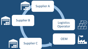
8.4.4 Milk Run Pick-Ups: A Special Case in Inventory Management
In certain sectors, particularly in industries like automobile manufacturing, the dynamics of inventory management take on a unique form known as “milk run pick-ups.” This method is especially prevalent in scenarios where:
- The demand for components is relatively uniform and predictable.
- Suppliers are located in close proximity to the main assembly or manufacturing plant.
In a milk run pick-up system, a truck departs from the main assembly plant at fixed intervals, say every two hours. This truck follows a predetermined route, visiting a specific set of suppliers. At each supplier, the truck picks up the required components and then transports them back to the factory. The name “milk run” is derived from the historical practice of milk delivery, where a milkman would follow a consistent route to pick up milk from various dairies and deliver it to homes or businesses.
This system offers several advantages:
- Predictability: Since the pick-ups are scheduled at regular intervals, suppliers can plan their production schedules accordingly, ensuring that components are ready for pick-up when the truck arrives.
- Efficiency: The fixed route and schedule eliminate the need for placing individual orders, reducing administrative overhead and streamlining the procurement process.
- Reduced Inventory: As components are delivered at regular intervals, the assembly plant can maintain lower inventory levels, relying on frequent replenishments.
Milk run pick-ups exemplify how inventory management strategies can be tailored to fit the specific needs and conditions of an industry, optimizing both the supply chain and production processes.
