10.2 Decision Trees

To illustrate the analysis approach, a decision tree is used in the following example to help make a decision.


Example 10.1

Product decision. To absorb some short-term excess production capacity at its Arizona plant, Special Instrument Products is considering a short manufacturing run for either of two new products, a temperature sensor or a pressure sensor. The market for each product is known if the products can be successfully developed. However, there is some chance that it will not be possible to successfully develop them. Revenue of $1,000,000 would be realized from selling the temperature sensor and revenue of $400,000 would be realized from selling the pressure sensor. Both of these amounts are net of production cost but do not include development cost. If development is unsuccessful for a product, then there will be no sales, and the development cost will be totally lost. Development cost would be $100,000 for the temperature sensor and $10,000 for the pressure sensor.

Figure 10.1 Special Instrument Products decision

Question 10.1: Which, if either, of these products should Special Instrument Products attempt to develop?

To answer Question 10.1 it is useful to represent the decision as shown in Figure 10.1. The tree-like diagram in this figure is read from left to right. At the left, indicated with a small square, is the decision to select among the three available alternatives, which are 1) the temperature sensor, 2) the pressure sensor, or 3) neither. The development costs for the develop temperature sensor and develop pressure sensor alternatives are shown on the branches for those alternatives. At the right of the development costs are small circles which represent the uncertainty about whether the development outcome will be a success or a failure. The branches to the right of each circle show the possible development outcomes. On the branch representing each possible development outcome, the sales revenue is shown for the alternative, assuming either success or failure for the development. Finally, the net profit is shown at the far right of the tree for each possible combination of development alternative and development outcome. For example, the topmost result of $900,000 is calculated as $1 000 000 ¡ $100 000 = $900 000. (Profits with negative signs indicate losses.)

The notation used in Figure 10.1 will be discussed in more detail shortly, but for now concentrate on determining the alternative Special Instrument Products should select. We can see from Figure 10.1 that developing the temperature sensor could yield the largest net profit ($900,000), but it could also yield the largest loss ($100,000). Developing the pressure sensor could only yield a net profit of $390,000, but the possible loss is limited to $10,000. On the other hand, not developing either of the sensors is risk free in the sense that there is no
possibility of a loss. However, if Special Instrument Products decides not to attempt to develop one of the sensors, then the company is giving up the potential opportunity to make either $900,000 or $390,000. Question 10.1 will be answered in a following example after we discuss the criterion for making such a decision.

You may be thinking that the decision about which alternative is preferred depends on the probabilities that development will be successful for the temperature or pressure sensors. This is indeed the case, although knowing the probabilities will not by itself always make the best alternative in a decision immediately clear. However, if the outcomes are the same for the different alternatives, and only the probabilities differ, then probabilities alone are sufficient to determine the best alternative, as illustrated by Example 10.2.

Example 10.2

Tossing a die. Suppose you are offred two alternatives, each of which consists of a single toss of a fair die. With the first alternative, you will win $10 if any number greater than 4 is thrown, and lose $5 otherwise. With the second alternative, you will win $10 if any number greater than 3 is thrown, and lose $5 otherwise. In this case, since there are 6 faces on a die, the probability of winning is [latex]\frac{2}{6}[/latex] = [latex]\frac{1}{3}[/latex] for the first alternative and  [latex]\frac{3}{6}[/latex]= [latex]\frac{1}{2}[/latex] for the second alternative. Since the consequences are the same for both alternatives and the probability of winning is greater for the second alternative, you should select the second alternative.

However, the possible outcomes are often not the same in realistic business decisions and this causes additional complexities, as illustrated by further consideration of the Special Instruments Product decision in Example 10.3.


Example 10.3

Product decision. Suppose that in Example 10.1 the probability of development success is 0.5 for the temperature sensor and 0.8 for the pressure sensor. Figure 10.2 is a diagram with these probabilities shown in parentheses on the branches representing the possible outcomes for each sensor development effort. (While only the probability of success is specified for each development effort, the probability of failure is determined by the rules of probability since the probabilities of development success and development failure must add up to one.) A study of Figure 10.2 shows that having the probabilities does not resolve this decision for us. The figure shows that although the probability of development success is considerably lower for the temperature sensor than it is for the pressure sensor (0.5 versus 0.8), the net profit from successful development of the temperature sensor is considerably higher than the net profit from successful development of the pressure sensor ($900,000 versus $390,000). That is, the alternative with the higher potential payoff has a lower probability that this payoff will actually be realized.

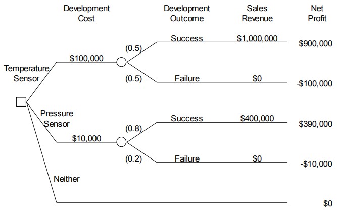
Figure 10.2 Special Instrument Products decision tree

The resolution of this decision dilemma is addressed in the next section, but before doing this, Definition 10.1 clarifies the notation in Figures 10.1 and 10.2.

Definition 10.1: Decision tree notation

A diagram of a decision, as illustrated in Figure 10.2, is called a decision tree. This diagram is read from left to right. The leftmost node in a decision tree is called the root node. In Figure 10.2, this is a small square called a decision node. The branches emanating to the right from a decision node represent the set of decision alternatives that are available. One, and only one, of these alternatives can be selected. The small circles in the tree are called chance nodes. The number shown in parentheses on each branch of a chance node is the probability that the outcome shown on that branch will occur at the chance node. The right end of each path through the tree is called an endpoint, and each endpoint represents the final outcome of following a path from the root node of the decision tree to that endpoint.


Attribution

By Craig W. Kirkwood, Chapter 1 of Decision Tree Primer,  January 11, 2013, licensed under a Creative Commons Attribution License CC BY-NC-SA 4.0.

License

Icon for the Creative Commons Attribution-NonCommercial-ShareAlike 4.0 International License

Data Analytics for Public Policy and Management Copyright © 2022 by Luis F. Luna-Reyes, Erika G. Martin and Mikhail Ivonchyk is licensed under a Creative Commons Attribution-NonCommercial-ShareAlike 4.0 International License, except where otherwise noted.

Share This Book