12.3 Using Excel to Solve Optimization Problems
Excel has a routine to solve LP problems called “solver,” and in this section of the chapter we will show haw to use this functionality to solve a LP problem.
Setting the Spreadsheet
Setting up a LP problem in Excel is quite simple once the model has been defined as described in the previous section of the chapter. Figure 12.3 shows a potential setting for the Farmers problem in Excel. Besides a special area to capture all the inputs to the problem (cost, time, profit), all other areas in the spreadsheet correspond to the three key elements of a LP problem, the Objective Function, the Decision Variables and the Constraints.
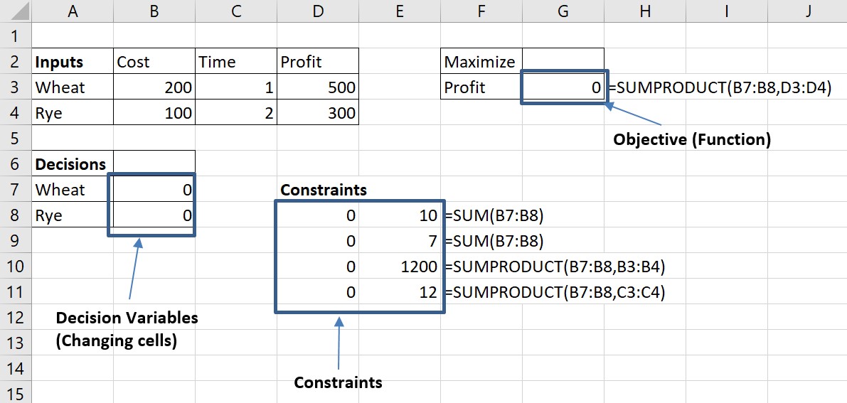
Figure 12.3 LP MOdel setting in Excel
To set the inputs in the model, the constants provided in the text were entered into the spreadsheet with toe proper labels. The Decision Variables in the model were assigned zeroes as an initial value. Solver will find the actual solution, and it is possible to enter in these cells any value.
To enter Constraints and Objective Functions, it is possible to use the functions =SUM() and =SUMPRODUCT(), which are the best Excel functions to represent linear functions. When the function follows the form W + R –without any coefficients to the decision variables– it is possible to enter the equation as =SUM(), and when the equation follows the form C1W + C2R –where Ci represents any coefficients in the equation– it is possible to use the function =SUMPRODUCT(). The example in Figure 12.3 includes each of the equations included in the model from previous section. For profit, that we modeled as Profit = 500W + 300R the Excel model uses then =SUMPRODUCT(B7:B8, D3:D4), B7 and B8 are the decision variables W and R, and D3 and D4 include the constants 500 and 300. All other constraints, included in D8 to D11 use the equations at the right of the numbers.
Using Solver to Find the Solution
Once the LP model is set in an Excel Spreadsheet, it can be solved by entering the three main components into the Excel Solver Window (Figure 12.5). To open the Solver Window, you need to choose the option in the “Data” tab in Excel. The solver button is usually at the extreme right side of the ribbon (see Figure 12.4). When the Solver button is not visible in the Ribbon, it is most likely that the Solver Add-in needs to be activated in your computer. To activate the Solver Add-in, you will need to choose “Options” in the “File” menu in Excel, go to the Add-ins panel and click on the “Go” button to manage the Excel Add-ins. Make sure that the option for the Solver Add-in is selected as it is shown in Figure 12.4.
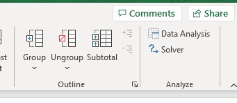
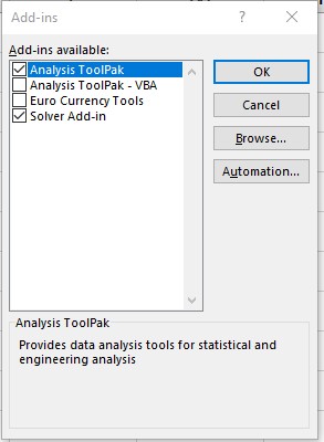
Figure 12.4 Solver button and Add-ins window in Excel.
As it is hown in Figure 12.5, there are three main spaces in the Solver Parameters Window to enter the Objective Function (Set Objective), the Decision Variables (By Changing Variable Cells) and the model Constraints. To add the objective function cell, it is possible to enter it manually, but it is also possible to click on the arrow at the right of the space for the function, and then click on the cell where the objective function is located. Same process applies to enter the Decision Variables.
To add the Constraints into the model, click on the “Add” button to display the window at the right of Figure 12.5. You can enter each constraint by clicking again on the appropriate cells in the spreadsheet. Make sure that the simbol in between cells is the appropriate for each constraint and click add. Once you added the last constraint, click on OK to close the window.
Make sure to check the “Make Unconstrained Variables Non-Negative” option to include the non-negativity constraints when appropriate, and make sure to choose the “Simplex LP” method as the solving method. Once the model is set, click on Solve and Excel will provide a solution.
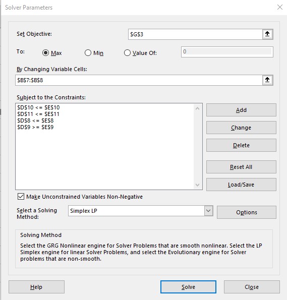
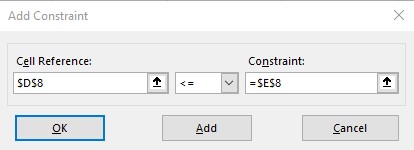
Figure 12.5 Solver and Add constraint Windows
After clicking the “Solve” button, Excel will make calculations and will show a window with the result of the process, explaining that it was possible (or not) to find a solution. Click OK and look at the numbers in the spreadsheet (Figure 12.6). All zeroes have changed to the actual numbers for solutions, constraints and objective. The farmer will maximize their profit planting 4 acres of Wheat and 4 acres of Rye. The actual profit is $3,200, and they are using 8 acres, all the money and all the time. Any other combination within these constraints will result in a lower profit.
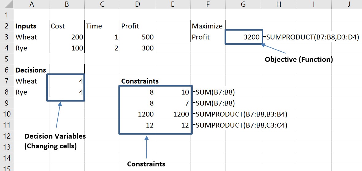
Figure 12.6 Solution to the Solver
Rmember the Steps to solve an LP Problem
- Understand the problem.
The goal of a linear programming problems is to find a way to get the most, or least, of some quantity — often profit or expenses. This quantity is called your objective function. The answer should depend on how much of some decision variables you choose. Your options for how much will be limited by constraints stated in the problem. - Describe the objective.
What are you trying to optimize? Are you trying to minimize costs? Maximize production quantities? You may have constraints like “you can’t spend more than $1000” or “you mus’t ship at least 50 tons of product C”. These are limits but don’t necessarily reflect your employer’s top priorities; don’t mistake these for suggestions that you minimize costs or maximize production. - Define the decision variables.
The answer to a linear programming problem is always “how much” of some things. What are those things? Choose variables to represent how much of each of those things. - Write the objective function.
Use the variables you just chose to write down an algebraic expression that describes the amount you’re trying to minimize. - Describe the constraints.
What are the limits on “how much” your decision variables can be? Look for words like “at least”, “no more than”, “two thirds of”, “we must fill orders for”, etc. - Write the constraints in terms of the decision variables.
For each constraint such as “at least $500” or “no more than 29” write an inequality using the decision variables. - Add the nonnegativity constraints.
Don’t forget to include non-negativity constraints like P >= 0. These are worth a quick two points on the quiz. - Set up the Problem in Excel.
- Use Solver to find a solution.
Attribution
By Luis F. Luna-Reyes, Erika Martin and Mikhail Ivonchyk, and licensed under CC BY-NC-SA 4.0.
