Core Concepts

MAUT models are tabular comparisons of decision choices and the way they meet a set of objectives or criteria. As it is shown in Figure 11.1, It is common to arrange MAUT models with the alternatives or decision choices as column headers and the criteria or objectives as row headers. In the warming-up problem, Prueba, Valora and Evalua are the three main alternatives under analysis. Efficiency, percentage of error and cost, on the other hand are the main goals or criteria that decision makers are using to compare the three alternatives. Finally, the contents of the table are commonly described as consequences. In other words, if the decision maker chooses Valora, Inc., the consequences of their decision are to have a response time of 2 days, a % of error of 0.008 and a cost of 10 dollars.

Figure 11.1 Core elements of a MAUT Model

It is important to note that objectives (or criteria) are personal and the selection of them respond to the values of the decision maker. As such, we need to be thoughftul in their selection, and when working on a business decision, intentional in covering the interests of all your stakeholders when choosing the objectives. Objectives are also valuable because they are useful in identifying new potential alternatives by thinking on different ways of attaining those objectives.

A second important note relates to the consequences, which are key data elements in the model that are usually the result of research performed by an analyst. The first note is that –just as any other data element in a model– they can come in both numeric and textual form, and an analyst should be open to have both qualitative and quantitative information about consequences of choices. A common mistake involves the elimination of important goals only on the basis of having no access to quantitative information on the consequences of them. The MAUT process described in the following paragraphs is useful for both quantitative and qualitative consequences.

The Multi-Attribute Problem

A major difficulty of making decisions using multiple goals or criteria is that most likely we will not be able to find a clearly superior alternative. In the initial example, Valora labs are the fastest, Evalua are the cheapest, and Prueba are the best in quality. As you were thinking about the best alternative for this problem, you faced an old decision problem known as the multi-attribute problem. There are two main components to the problem. The first component relates to the difficulty of having many goals or criteria measured in different scales. In selecting a lab to run the tests we had three different types of information coming in different scales and units (days, %, dollars), making it difficult to compare and make trade-offs using those numbers. Having criteria that uses different scales and units makes it difficult to simply add them up to assess the potential value of each alternative. The second component of the multi-attribute problem –assuming that we solve the first– involves figuring out a rule to be able to use all measures simultaneously in choosing an alternative. In other words, how do we use all the information at the same time reflecting our priorities for each goal?

Researchers on decision making have developed many approaches to solve this problem. Examples of these approaches include the use of value functions, simple additive weighting, pairwise comparison or distances to the ideal solution, among many others. In this section of the chapter, we are going to learn one intuitive approach that follows in the family typically known as Multi-attribute Utility Theory or MAUT. Note that MAUT approaches are best to situations that involve discrete alternatives, i.e. we can count and differentiate those alternatives. In the next chapter we will learn about Linear Programming, a method used for continuous problems, where the number of alternatives is infinite. Let’s start with some basic concepts and a simple approach that uses MAUT to find a recommendation for the Mayor on the lab selection problem.

Steps to Develop a MAUT Model

Building a MAUT model involves many steps starting with a clear definition of the decision problem, establishing goals or criteria that need to be met, identifying alternatives and researching the consequences for each alternative (see below). In this section of the chapter, however, we will focus first on steps 5 and 7, normalizing the data and calculating a simple utility score to compare the alternatives. These steps also constitute one possible path to solve the multi-attribute problem. We are going to use Microsoft Excel to set up the model in a computer, using that model to make it more complex and explore the robustness of the decision in the following sections of the chapter.

Normalizing data

The first step providing a solution to the muli-attribute problem consists on the development of a normalized scale that can then be used to compare all the alternatives. This normalized scale solves the problem of having different scales and units across criteria, making them more comparable. Normalizing values in this context refers to the idea of using a standard scale for all criteria. We suggest to use a simple scale that goes from zero to 100, and let’s say that those represent utility units. In this way, alternatives with the most utility units are better compared to the others. Let’s start by setting up the model in Excel. We will use the warm-up exercise as the core example for this procedure. There are at least two different ways of setting up a MAUT model in Excel as it is shown in Figures 11.2 and 11.3. Both possible configurations include the initial information included in the model and spaces to transform the scales into normalized values. In Figure 11.2, we created a row between each objective to include the new normalized scale. Figure 11.3, on the other hand, creates a whole new table that will include only the normalized values.

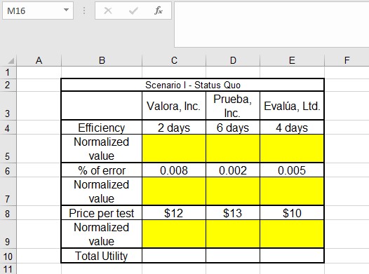
Figure 11.2 Alternate setting of a MAUT model in Excel

Figure 11.3 Alternate setting of a MAUT model in Excel

There are many different approaches to transform numbers into normalized values. For the purposes of this chapter, we will only include 2, using linear normalization, and a second approach using the decision maker judgment. Let’s start with the linear normalization.

Linear Normalization

The linear normalization approach involves the assumption that the utility value increases in a constant way. We need to different equations to transform the scales into a normalized scale given that for some objectives higher values are better, and for some others smaller values are better. For example, when looking at the cost of lab tests, or the efficiency in days in our warming-up example, smaller values provide more utility than higher values. Nonetheless, when comparing warranties from a vendor, more time will provide more utility. In this way, we can use the following two equations to normalize numaric scales.

If a higher value is preferred: [latex]\frac{\text{score - minimum}}{\text{maximum - minimum}}*100[/latex]

If a lower value is preferred: [latex]\frac{\text{maximum - score}}{\text{maximum - minimum}}*100[/latex]

Figure 11.4 includes a graphical depiction of the assumption, and the same two equations introduced above in a more “Excel” friendly version. The chart on top of the figure shows the basic assumption of the linear normalization (constant increase in utility. In this way, when higher values provide more utility, the highest value will become 100, the lowest value will become zero, and the values in between will take the value on the Y scale that corresponds to the value in the X scale. For cases where lower is better, the equation will act in the opposite way, transforming into 100 the lowest value and into zero the highest. Figure 11.4 also shows the way in which the equations above could be translated into an Excel formula. The very last line includes the full translation for cell C20 in the model presented in Figure 11.3.

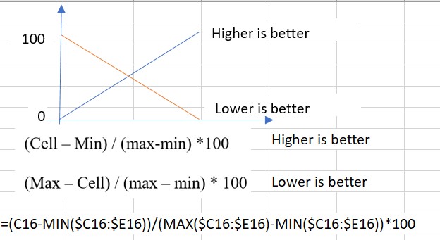
Figure 11.4 Linear Normalization in Excel

One advantage of the setting introduced in Figure 11.3 is that it allows for copying and pasting the equation in all the table, normalizing all values in a fast way. Absolute and relative values in the equation are already set in a way that copying is possible. Figure 11.5 includes the final result of the normalization process (noticed that the word days was erased from the model efficiency criteria to make the equation work).

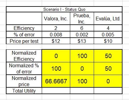
Figure 11.5 Normalized values.

Qualitative Normalization

As you may be thinking now, assuming that utility increases in a constant way may not always be a reasonable assumption. Utility may reduce faster when resources are limited or under emergency situations. Experts in decision making have developed many alternative equations to change this assumption. A second approach to normalization that can also be more flexible on this assimption consists of the use of qualitative judgments by the decision maker in the normalization process. These are the basic steps:

1. Identify the best and worse alternative to each objective and mke the Best=100, and the Worse=0
2. Assess qualitatively all other alternatives using the same 0-100 scale.

Figure 11.6 includes the model in Figure 11.2 using this alternate qualitative approach. It also includes possible ways in which the qualitative judgement can modify the linear assumption. In the case of efficiency, utility changes faster than the linear example, and then instead of assigning the value of 50 to Evalua, they only get a 20. In the case of price of the test, on the other hand, utility changes slower than in the linear case, and Valora gets 85 utility points instead of 66.67. Notice that the best and the worst values get the utility of zero and 100 in both approaches. Having those anchors in the utility scale makes this normalized scale most useful for comparison purposes.

Figure 11.6 Qualitative Normalization results.

Comparing Alternatives

After normalizing the scales for each objective in the MAUT model, the next step is to compare the alternatives. The simplest way of comparing alternatives is just to add the new normalized scales. Given that all these new scales are in utility units, the alternative with the highest numer is the one that provides more utility value to the decision maker, becoming the recommended option. Figure 11.7 includes the final model with the qualitative judgments. According to this model, Valora, Inc. is the recommended alternative given that this one offers the most utility. Using this simple approach assumes that all objectives have the same importance for the decision makers. In the following section, we will introduce a simple approach to assign different weights to each objective or criteria.

Figure 11.7 MAUT Model with total Utility

Attribution

By Luis F. Luna-Reyes, Erika Martin and Mikhail Ivonchyk, and licensed under  CC BY-NC-SA 4.0.