12.2 Linear Programming Core Concepts
As briefly described in the introduction to the chapter, linear programming (LP) is a mathematical technique that can be used to find optimal solutions to decision problems that can be expressed using linear equations and inequalities. Typical situations that involve the use of linear programing include decision problems where we are looking for optimal resource allocation. Although only few problems can be perfectly represented through linear equations and functions, many more problems can be assumed to be linear in a more or less realistic way. As any other modeling technique, LP offers an approach to think about a complex problem in a reasonable way to get a better understanding of the solution space. LP models are also useful when certainty can also be assumed.
To better understand the concept of a linear function or equation, please consider the following examples.
Examples of Linear Situations
- Prof. Luna-Reyes takes 30 minutes to grade 1 midterm, and 4 hours to grade 8 midterms
- Paul needs 5 minutes to process each online toy tractor order
- Each acre of wheat costs $200 to plant
- Each acre of rye cost $100 to plant
- Total cost to plant rye and wheat
All examples of a linear fonction provided in the box assume a constant use of the resource every time that we process one item, there is no efficiencies produced by volume, diminishing returns or learning curves. In this way, linear functions can be modeled as combinations of sums and multiplications of constant resource use. The following box includes examples of such linear functions. All functions in the example box are linear functions.
Examples of Linear Functions
- Prof. Luna-Reyes takes 30 minutes to grade 1 midterm (M), and 4 hours to grade 8 midterms: Time Grading = 30M
- Paul needs 5 minutes to process each online toy tractor (T) order: Time Processing = 5T
- Each acre of wheat (W) costs $200 to plant: Wheat Cost = 200W
- Each acre of rye cost (R) $100 to plant: Rye Cost = 100R
- Total cost to plant rye (R) and wheat (W): Total cost = 100R + 200W
As you may imagining now, non-linear situations are all those in which the use of resources is not constant given the effect of added efficiencies, learning curves or effects of getting tired or diminishing returns. Some examples of these non-linear situations include the following.
Examples of Non-Linear Situations
- It takes Prof. Martin 1 hour to bike 20 miles, but 2.5 hours to bike 40 miles (she gets tired and can’t maintain the pace!)
- It takes Prof. Luna-Reyes 2 hours to cook the Thanksgiving meal for his wife and daughters, but only an additional 30 minutes (2.5 hours) to double the portions so that he can also feed his parents and in-laws (economies of scale)
Modeling these situations involves the use of non-linear functions and equations. Non-linear equations include all mathematical expressions where the analyst use exponents, roots, variables in the denominator or other mathematical functions such as logarithmic and exponential functions.
Main Components of a Linear Program
Modeling a decision using LP involves the identification of three core components: (1) the decision variables, (2) the objective function and (3) the main constraints. We will use the warming-up exercise to exemplify each of these components.
The answer to a linear programming problem is always “how much” of some resources. These resources are the decision variables. Identifying those resources is an important componenet of any linear programing problem, and any combination of those resources is a potential solution to the problem. For example, in the case of the farmer in the warming-up problem, we can say that the decision variables are two: R or how many acres of rye to plant and W or how many acres of wheat to plant. You may find useful to name these variables using letters. Any combination of these 2 is a potential solution. The farmer can plant R=2 and W=8 or R=4.5 and W=3.5. Any combination of acres is a potential solution, and you may start to see how the number of alternative solutions is not discrete, and involves many potential solutions (infinite in fact).
The goal of a linear programming problems is to find a way to get the most, or least, of some quantity — often profit or expenses. This quantity is called the objective function. Which alternative is the best one depends on this objective of the decision maker. The answer should depend on how much of some each decision variables you choose. In our initial problem, the goal is to capture the highest possible profit from farming. Given that we know that each acre of Rye (R) will produce $300 profit and each acre of Wheat (W) will produce a $500 profit, we can define the objective function for the farmer as Profit = 500W + 300R, which is a linear function. Every choice is associated to a specific profit. If we choose, for example, R=2 and W=8, the expected profit will be 500(8) + 300(2) = 4,600.
Although it could seem reasonable to choose planting all 10 acres of wheat because it is the one providing the highest profit per acre, our options are usually limited by the availability of resources, which is usually limited. These limited resources are commonly named constraints, the third component of a LP problem. In this way, identifying what are the limits on “how much” your decision variables can be constitute the constraints of the problem. In our initial problem, there are 3 main resources, land, money and time (maybe associated with the use of equipment). The farmer can plant any combination of acres, but they have only 10 acres to plant, and they must plant at least 7 acres. The second constraint is a limited amount of money ($1,200), and the given cost of planting each acre, which is $200 per acre of wheat and $100 for each acre of rye. The final constraint is time, the farmer have only 12 hours to plant, and each acre of rye will take 2 hours to plant and each acre of wheat will take 1 hour to plant. These constraints can be also expressed as linear functions of the two main decision variables. It is most common to use the symbols <, >, <= and >= to these constraints, given that they can be any combination of values up to each constrained resource, or using at least some amount of each resource. In the case of our initial problem, we can establish the four constraints as two land constraints W + R <= 10 and W + R >= 7, a money constraint 200W + 100R <= 1,200 and a time constraint, 1W + 2R <= 12. Given that most policy decisions include only positive numbers (we cannot plant negative acres), it is common to add also non-negativity constraints for each decision variable, R>=0, W>=0.
A LP program is commonly expressed then in the following way :
| Maximize | Profit = 500W + 300R |
| Subject to constraints: | W + R <= 10
W + R >= 7 200W + 100R <= 1,200 1W + 2R <= 12 R >= 0, W >= 0 (non-negativity constraints) |
| Where | R – Acres of Rye
W – Acres of Wheat |
A Graphical Representation of a Linear Programming Problem
When a linear programming problem involves only two decision variables it is more or less simple to translate the problem into a set of lines and surfaces in a coordinate system, and that picture may be useful to better understand the LP model, the solution space and the potential solutions.[1] Each of the inequalities in our warming-up problem can be represented in a coordinate system as a plane. Figure 12.1 includes the first land constraint in our problem. Any point in the shaded area in the figure, including points on the line, constitutes a solution to the inequality W + R <= 10. In other words, any point in the shaded area will make the inequality true. For example, the point (2,2) in the inequality would be 2 + 2 <=10, which is true.
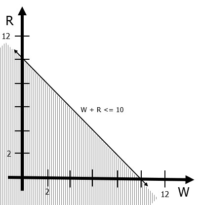
Figure 12.1 Graphical representation of W + R <= 10
Nonetheless, the area represented in Figure 12.1 is only one of the cnstraints in the problem, and to figure out the solution space –all possible decisions– it is necessary to graph all constraints and identify the area at the intersection of all the areas produced by the constraints. Figure 12.2 includes all four main constraints of the problem, identifying the solution space for the farmers problem as the small triangle at the center of all the lines. Optimal solutions in the space are located in the corners of the solution space, and for the farmer’s problem, the most profit can be found when they pland 4 acres of wheat and 4 acres of rye.
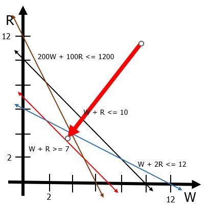
Figure 12.2 The Farmer’s Problem
Atribution
By Luis F. Luna-Reyes, Erika Martin and Mikhail Ivonchyk, and licensed under CC BY-NC-SA 4.0.
- Problems with three or more decision variables are harder to represent using graphs. Three decision variables need to be represented as planes in a three dimensional space, and more decision variables are impossible to graph in our three-dimensional world. ↵
