18
In this lab, we’re going to learn how conduct a dependent t-test, also known as a paired t-test or repeated measures t-test, using SPSS. For this lab, we’ll be exploring global climate data in the “US_Temperatures.sav” dataset. This dataset was created by generating a random list of 30 U.S. cities, using randomlists.com/random-us-cities, and then finding the mean annual temperature for each city in 1995 and in 2019 using NOAA’s Climate at a Glance: City Time Series (https://www.ncdc.noaa.gov/cag/). If a city was not listed on NOAA’s website or if the temperature data was incomplete, a nearby city was used.
First, open the dataset using SPSS. You’ll notice this dataset has four variables: the city name, the state where the city is located, the mean annual temperature in 1995, and the mean annual temperature in 2019. This data would be appropriate for a dependent t-test because we are exploring the difference between two variables that can each be paired up with the same case. Very often, variables in dependent t-tests are observations at different times as in our example. In other cases, you might have participants that are tested more than once, perhaps to determine the efficacy of a medical treatment, for example.
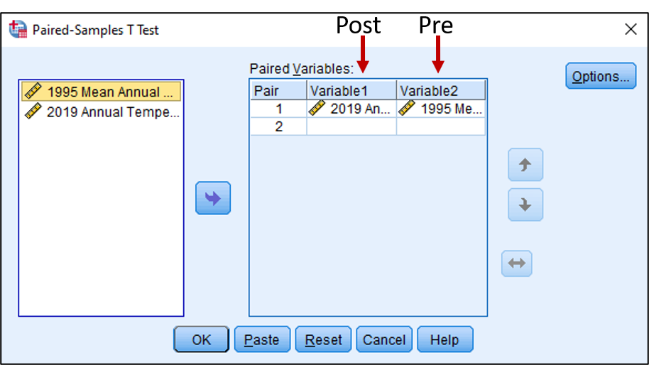
To conduct a dependent t-test, click Analyze, then Compare Means, then Paired Samples T Test. A Paired Samples T Test dialog box should appear. Drag the variable “1995 Mean Annual Temperature” to the “Variable2” space. Please note, in SPSS, the pre-test variable or the oldest time series should always go in the Variable2 space because SPSS calculates the t-test using Variable1 minus Variable2, or Post minus Pre. Drag the variable for “2019 Mean Annual Temperature” into the “Variable1” space. Click OK.
Three tables should now appear in your SPSS Output Viewer window. Notice in the “Paired Samples Statistics” box, there is a mean value for each of our variables. In 2019, the overall mean temperature of our sample was 61.33 degrees Fahrenheit, while in 1995 it was 60.367. This does not seem like a substantial increase, but what the dependent t-test explores is whether or not this increase is statistically significant. In other words, did we generally see temperatures increase across all cities in our sample?
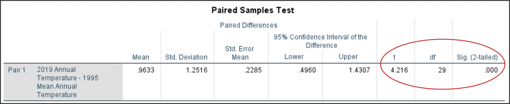
The results of the dependent t-test are located in the “Paired Samples Test” box. What is the value of the t-statistic? Look in the “t” column. In our case, the value is 4.216. What would the critical value of t be for our dataset? You’ll notice the degrees of freedom are located in the “df” column, which is 29 (the number of paired samples, n, minus 1.) Look up the critical value of t in your statistics book or using an online calculator. Is this obtained value of t more extreme than the critical value?
What is the significance? This result can be found in the column labeled “Sig. (2-tailed).” You’ll note that this value is .000. Does this mean the value should be reported as zero? If you double-click this table to activate it, you can hover over the significance value in the new window that appears. You’ll see the actual value is 0.000222. Is this less than 0.05? Very much so. Thus, we can conclude that there was a significant increase in temperatures from 1995 to 2019. The p-value can be reported as “p<.01.”