23
There are a number of different tests a researcher could use to statistically analyze non-parametric data. One of the most common is the Chi-Square Test of Independence. This lab will teach you how to conduct a Chi-Square Test of Independence using SPSS. We will be using the “Religion.sav” dataset. This dataset contains a sampling of data from Pew Research Forum’s American Trends Panel, Wave 54, conducted in September of 2019. The entire dataset can be accessed here: https://www.pewsocialtrends.org/dataset/american-trends-panel-wave-54/. For our example, we’re only exploring a few of the dozens of variables in Pew’s dataset.
First, open the dataset using SPSS. Note that we have four variables, and the name of each is capitalized and sometimes abbreviated. This is common in larger datasets. Click on the “Variable View” tab to view the full labels for each variable and click the value labels area to expand and browse the numeric codes used to represent different responses. If you open a dataset and find this information isn’t provided, or there aren’t labels provided for abbreviated variable names, check for a “Codebook” which often accompanies large datasets and will provide this information. We’re working with a lot more respondents than we’re used to. You’ll see there are 6,679 cases in this dataset, each representing one survey respondent. The original dataset is larger, but for this example, respondents with missing or incomplete data have been removed.
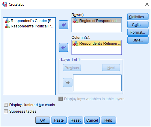
Let’s investigate the relationship between religious affiliation and the respondent’s region. Are certain religions more likely to be found in particular regions of the United States? To run a Chi-Square test with SPSS, click on Analyze, then Descriptive Statistics, then Crosstabs. Crosstabs, or cross-tabulations, simply refer to tables showing the relationship between categorical variables. In the Crosstabs dialog box that appears, select “Region of Respondent” and move it to the “Row(s)” box. Select “Respondent’s Religion” and move it to the “Column(s)” box. Next, click the Statistics… button and check the box next to “Chi-square” since this is the test we’re going to run. Click Continue. It would also be helpful to view percentages for our data and not just the frequency counts, so click the Cells… button and then in the “Percentages” area, check all three boxes: Row, Column, and Total. Click Continue and then click OK.
In our Output Viewer window, we should see three tables. The first is the Case Processing Summary. This table is very helpful when working with large datasets because it shows us the number and percentage of cases which were valid and which were missing. Sometimes, you might find an interesting variable but a majority of data is missing. Perhaps respondents declined to answer that question in large numbers. We see that we have a sample size of 6769 respondents with no data missing (again, because this dataset has been cleaned and some of the respondents with missing data have been deleted.)
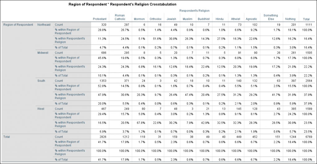
Next, we see our Crosstabulation. Here you can find the frequency values (listed in the “Count” rows) for each of our pairs. For example, Protestant respondents who live in the Northeast, Roman Catholic respondents who live in the Midwest, and so on. We also see the percentages of these values both within the region and within the religion. This can be a little confusing to break down, so let’s look at the numbers a moment. 320 Protestant respondents live in the Northeast region (as you can find in the cell next to “Northeast Count” and under “Protestant.” The percentages listed in this section note that 28.8% of all respondents who live in the Northeast were Protestant (% within Region of Respondent) and 11.3% of all Protestant respondents live in the Northeast (% within Respondent’s Religion).
Finally, we have the results of our Chi-Square test.
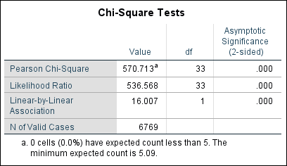
The value of Chi-Square is 570.713 and the significance is less than .05, which indicates that there is a significant relationship between a respondent’s religion and the region where they live. Note also that there is a footnote below the Chi-Square Tests table, indicating that in our dataset, no cells have an expected count less than 5. One assumption of the Chi-Square test is that no more than 20% of the cells should have expected values less than 5 and we have not violated this assumption.
What other relationships exist in our data? Try to pair different variables and see if you can find any other relationships that are statistically significant.
