20

In this lab, we’ll learn how to compare means when we have more than two groups, which is known as Analysis of Variance (or ANOVA). This example will walk us through one-way ANOVA, also known as simple ANOVA. We will be using the “US_Income_Inequality.sav” dataset, which contains the Gini coefficient value for each state in the United States. The Gini coefficient is a measure of income inequality within a population. A Gini coefficient of 1 (or 100 percent) would mean that a group of people is an unequal as it could possibly be, with one person holding all the wealth and all others having none. Conversely, a Gini coefficient of 0 would mean that everyone is perfectly equal in a society with regards to income. Nationwide, the Gini coefficient across the entire United States in 2016 was 41.50 percent, or .415. This data has been compiled using information from the Population Reference Bureau (https://www.prb.org/usdata/indicator/gini/table), which compiles data gathered from U.S. Census Bureau, American Community Survey.

First, open the dataset using SPSS. You’ll notice there are three variables: the state name, the Gini coefficient (expressed as a percentage), and the region code. The region codes are utilized by the U.S. Census bureau. If you click on the “Variable View” tab, look at the Region row and click on the “Values” column and then the … button. Here, you can view the various labels for the region codes. There are four regions defined by the Census: Northeast, Midwest, South, and West.

This dataset would be appropriate for one-way ANOVA because we have one variable we’re comparing, in this case the Gini coefficient, and we have more than two different groups (in our case, we have four different regions.)

To conduct one-way ANOVA, click Analyze, then Compare Means, then One-Way ANOVA. A “One-Way ANOVA” dialog box should appear. What is our dependent variable? The Gini coefficient, because we’re curious whether income inequality is dependent on region. Move “Gini” over to the “Dependent List” by clicking the variable and then clicking the arrow next to the “Dependent List” box. What is the factor? Factor refers to the independent variable, or group. In our case, it’s the state’s region, so move “Region” to the Factor box.

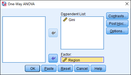
We have a couple more options to select before we run our test. Click on Options… and then click the check box next to “Descriptives.” Click Continue. Lastly, click Post Hoc… and then click the check box next to “Bonferroni.” This will allow us to not only determine if there is significance variance somewhere in our data but, critically, where this variance is among our groups. Click Continue.

Back in the One-Way ANOVA dialog box, click OK to run our test. In the Output Viewer window, you should see several different tables. The first is our Descriptives table, where we can find general descriptive statistics for each of the four regions. Next is the ANOVA table. So, is there a significant difference in income inequality between our four regions? Check the obtained F statistic and the significance value.

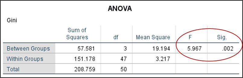
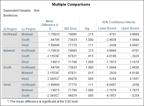
Our obtained F statistic is 5.967 and the significance is .002, so there certainly is a difference in income inequality between these regions. But where exactly is that difference? Since the result of our ANOVA test is statistically significant, we should check our post-hoc analysis, which is found in the table labeled “Multiple Comparisons.” The Bonferroni test is a simple post-hoc analysis that essentially uses multiple t-tests to compare differences between groups. Importantly, Bonferroni avoids a common error in running multiple t-tests by dividing the significance level between the number of comparisons made so that the cumulative total equals the original error rate selected. (This is why this test is sometimes called a Bonferroni correction.)

So where are there significant differences in our data? Significant differences between pairs are highlighted with an asterix (and this can be confirmed by determining where there are significance values less than .05). Note that significant differences exist between the Midwest and South and between the South and West. We could thus conclude that there is a significant regional variation in income inequality across the United States, with the most significant regional differences between the South and the Midwest and the South and West.