17
In this lab, we’re going to conduct an independent samples t-test using Excel. For this exercise, we’re going to be using the “Florida_Weather.xlsx” dataset, which contains historical weather data for 15 urban and 15 rural locations across Florida in November of 2020. The location classification was determined using maps from the USDA Rural Development program, available at https://eligibility.sc.egov.usda.gov/eligibility, and historical weather data from WeatherUnderground (https://www.wunderground.com/). First, open the file using SPSS.
You’ll notice that this file has five variables: the location name, the classification (rural or urban), the numeric classification code (0 for rural, 1 for urban), the total precipitation in inches in November 2020, and the average temperature that same month. This data is appropriate for an independent samples t-test because there are two distinct groups of data (rural and urban in this case) and we are interested in comparing the means of each group. As geographers, we might compare samples based on development level (comparing more developed and less developed countries, for example), social and demographic characteristics (perhaps gender or education level), or physical features (such as landcover.)
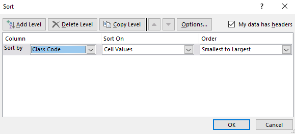
To conduct an independent samples t-test, we’ll use the Data Analysis toolpak. Let’s find out if there’s a significant difference in total precipitation between rural and urban areas. First, we’ll need to sort our data into groups. Highlight all of the data and then click Data, Sort, and then Sort by “Class Code.” Then, click OK.
Now, we have our data grouped by rural locations and then by urban locations.
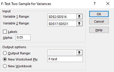
Before we run our t-test, we’ll need to check if our samples have roughly equal variances to determine which type of t-Test we can use. To do this, click on Data and then the Data Analysis button. In the dialog box that appears, click “”F-test Two-Sample for Variances.” Then click OK. In the dialog box that appears, select D2 through D16 as the Variable 1 range (all of the rural locations) and D17 through D31 as the Variable 2 range (all of the urban locations). Let’s create a new Worksheet for this test, so next to “New Worksheet Ply:” type: F-test. Then, click OK.
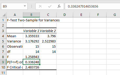
A new worksheet should appear with the results of the F-test, but how do you interpret this? You’ll note a cell labeled P and a value next to it. If you click this cell (cell B9), you’ll see the actual number in the formula box, which is 0.336… You’ll also notice that the variances for variables 1 and 2 appear to be fairly similar. If your p-value is less than 0.05 (and in our case, it is not), then we would reject the null hypothesis that the variances are equal. In our case, the variances are not significantly different. Our p-value is greater than 0.05 so we do not reject the null hypothesis. We can use the t-test for equal variances.
Now, go back to Sheet 1 and let’s compute our t-statistic. Click on Data and then Data Analysis. This time, scroll down to “t-Test: Two-Sample Assuming Equal Variances” and click it. Then click OK.
A new dialog box should appear. Follow the same steps as for the F-test: select D2 through D16 as the Variable 1 range and D17 through D31 as the Variable 2 range. Let’s create a new Worksheet for this test, so next to “New Worksheet Ply:” type: T-test. Then, click OK.
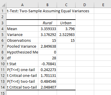
A new worksheet should appear with the results of our t-Test. You may have to resize column A to view all of the data labels. Re-label Variable 1 as Rural and Variable 2 as Urban. Just by comparing means, you can see that rural locations received less rainfall, on average, than urban locations. But the question is, is it significantly less? What is the value of the obtained t-statistic? It is -.708. We’ll use a two-tailed test, since we did not have prior knowledge about whether urban locations or rural locations would receive more rainfall. What is the critical value of the two-tailed t-statistic? It is 2.05. So, is our obtained value more extreme than the critical value? It is not, and we can confirm this by examining the p-value. Our obtained p-value is 0.48, which is not less than 0.05. This means we would not reject the null hypothesis and would conclude that the difference was not significant.
What if we compared temperatures rather than rainfall? Re-run the test and switch out “Average Temperatures” for the “Total Precipitation” variable and see if there’s a significant difference. Don’t forget to check for equality of variance using the F-test.
