1
In this lab, we’re going to get familiar with SPSS. It looks very similar to spreadsheet software you may have worked with before but has some important differences, so we’ll take some time to walk through it. First, open the file “Statistics_Course.sav.” Usually, you can click on a .sav file and it will open it with SPSS automatically, but if you have trouble, try opening SPSS first and then when the Welcome dialog box appears, click “Open another file…” under the “Recent Files:” area and navigate to the desired folder and file.
Once you’ve opened the file, you’ll notice that SPSS actually opens two windows, a Data Editor window and an Output Viewer window. Try to arrange them so you can see them both. A quick way to do this on a Windows computer is to hold the windows button and then hit one of the side arrow keys. Try it now. With your SPSS Data Editor window active, hold the windows button and hit your left arrow key. Your Data Editor window should now occupy the left half of your screen. Now, click in the Output viewer window to make it active and then hold the windows key and hit the right arrow key. It should now be next to your Data Editor. (Note, on newer versions of Windows, when you shift your Output viewer to the right, it might make the left side momentarily smaller and show a bunch of different possible windows you could select. Just select the Data Editor again.) This is a quick way to make any monitor a dual-screen monitor! If you’re working with a smaller monitor, just click between these two windows.
You’ll notice that the Data Editor looks similar to a spreadsheet while the Output Viewer is mostly blank space. Let’s start by exploring the Data Editor window.
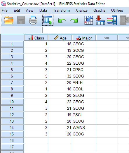
Within the Data Editor, there are two tabs: Data View and Variable View. Data View looks like a typical spreadsheet, but you’ll notice that the headings are fixed (whereas in Excel or Google Sheets, your headings are often just another row in the spreadsheet.) In SPSS, each row represents a particular case (or respondent) and each column represents a different variable. You’ll notice that in this dataset, we have 15 cases, each representing one student in a Quantitative Methods in Geography course. We also have three variables. Let’s click on the “Variable View” tab to see a longer description of each variable.
In the “Variable View” tab, we’ll see a description of each of our variables. The column “Name” refers to the name of the variable. Note that variable names in SPSS cannot begin with a number and cannot contain spaces. The “Type” refers to the type of data entered, such as Numeric, String (meaning text), Date, etc. “Width” refers to how much data can be entered in the cell – not to how wide the cell is in the Data View tab. “Decimals” is the number of decimals for numeric data. “Label” is a longer description of the variable, which is helpful when working with large datasets and considering the limitations for naming variables. For instance, what if you had a variable that referred to the number of times the respondent attends religious services each month? You might shorten this to “RelgAttend” in the variable name column, and then in the label column, write “Number of times respondent attends religious services each month.” The “Values” column provides the values of numeric codes for possible responses, which is often used for categorical or ordinal data. If you click on the cell in the “Values” column, you should see a … button appear, and you can click it to see the full list of values. Click on the top “Values” cell now to expand it.
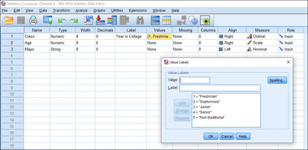
Here we have five different value labels, 1 to 5, each representing a different classification year in college. Click OK to exit out.
The column “Missing” refers to the values given to missing data. If a respondent chooses not to answer a question, it might be coded as 99, for example, or a period or a dash. These values should always be listed in the “Missing” column to ensure accurate calculations. “Columns” refers to the display width of the column. “Align” refers to how the data is aligned within the cell. Finally, “Measure” is one of the most important columns. This specifies the type of data in each variable and could be either scale (also known as interval), ordinal, or nominal (also called categorical.) The measure, or type of data, changes the look of graphs as well as the type of statistics that can be used to analyze the data, so it’s important that each variable measure is correctly set.
One handy tip, especially when working with large datasets, is to create a variable information table. Click on File, then Display File Information and then click Working File. Whenever you run a request in SPSS, you’ll find the results in your Output Viewer window. If you look at your Output Viewer window, you’ll see two tables: a Variable Information table and a Variable Values table. Here we a listing of all of our variables and, helpfully, a key for the values of the “Class” variable. Again, this can be very helpful when working with large, complicated datasets.
We’ll practice analyzing data in later labs, but for now, let’s just try to add a response. Let’s imagine we have another student to add to our dataset. This student is a Senior and is 22 and a Geography major. This will be our 16th case, so in row 16, under the Class column, type the number for the classification of Senior. (Go back to the “Variable View” tab if you forgot.) Next, type the student’s age in the next cell. Finally, type the four letter code used for the student’s major. That’s it!
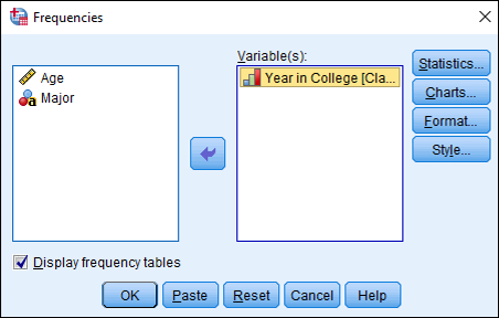
Lastly, let’s create a frequency table that includes our added response. Click on Analyze, then Descriptive Statistics, then Frequencies. A Frequencies dialog box should appear. Let’s break down our class by their year in school. Move this variable, “Year in College” over to the “Variable(s)” box either by double-clicking it or by clicking the variable and then clicking the arrow. Make sure there is a check in the box next to “Display frequency tables.” Finally, click OK.
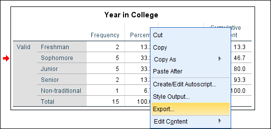
Notice our Data Editor hasn’t changed, so where is our table? In the Output Viewer window. Here we’ll find two tables, one noting N, our sample size, and how many values were valid and how many were missing. Below it, we’ll find our frequency table, listing all of the classifications and the number of students in each category in our class.
How can you save output in the Output Viewer? You could simply take a screen shot, but often the quality of screen shots isn’t great and they don’t resize well. A better option is to right click the table you’d like to save and click Export… A new window will appear with lots of options. At the top, you can decide which objects to export. Typically, you’ll just export the selected output. Under “Document,” select the Document type. Let’s select “Portable Document Format (*.pdf).” Check the save location next to “File Name” and browse to your preferred location if needed. Click the check box next to “Open the containing folder” and then click OK. This process may take a few seconds. You should see a PDF table of your Output. Nice work!
What if you want to copy your output into another document, perhaps a longer Word document where you’d like to use your output as a figure? You can also copy your Output as an image. Right click on the table you’d like to copy and click Copy As and then Image. In your Word document, right click and under “Paste Options,” click the Picture icon. (Or, in the Home tab, click the arrow under Paste and click the Picture icon.) Ta-da!
As you get more comfortable with SPSS, don’t be afraid to search online resources for help and tricks.
