16
In this lab, we’re going to learn how to run an independent samples t-test in SPSS. For this exercise, we’re going to be using the “Florida_Weather.sav” dataset, which contains historical weather data for 15 urban and 15 rural locations across Florida in November of 2020. The location classification was determined using maps from the USDA Rural Development program, available at https://eligibility.sc.egov.usda.gov/eligibility, and historical weather data from WeatherUnderground (https://www.wunderground.com/). First, open the file using SPSS.
You’ll notice that this file has five variables: the location name, the classification (rural or urban), the numeric classification code (0 for rural, 1 for urban), the total precipitation in inches in November 2020, and the average temperature that same month. This data is appropriate for an independent samples t-test because there are two distinct groups of data (rural and urban in this case) and we are interested in comparing the means of each group. As geographers, we might compare samples based on development level (comparing more developed and less developed countries, for example), social and demographic characteristics (perhaps gender or education level), or physical features (such as landcover.)
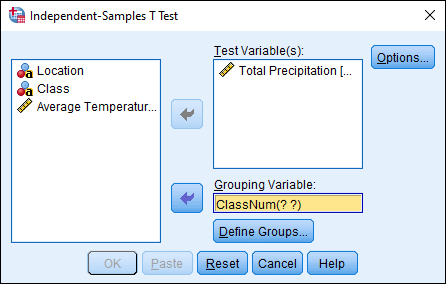
To conduct an independent samples t-test, click Analyze, then Compare Means, then Independent Samples T Test. An “Independent Samples T Test” dialog box should appear. First, let’s select our test variable. We’re curious if there are differing rainfall amounts for urban locations versus rural locations, so let’s move “Total Precipitation” to the “Test Variable(s)” box by clicking the variable and then clicking the arrow next to the “Test Variable(s)” box.
Next we should identify our “Grouping Variable.” This is the variable that specifies which group each particular case is in. In some datasets, your grouping variable might be a 0 or a 1, and you’ll need to check the “Values” column in the Variable View window to determine what those numbers represent. In other cases, you’ll only have a text string designating the group (such as developed, less developed.) For our example, we have both options available.
Click “Urban or Rural Numeric…” and then click the arrow next to “Grouping Variable” to move it into this box. You should see “ClassNum(? ?)” appear in the box. This means that we need to define our groups, so click on the Define Groups… button.
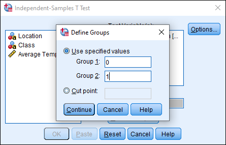
We’ll set Rural as Group 1 and Urban as Group 2, so type 0 in the Group 1 text box and 1 in the Group 2 text box. Note, if you only had string data for each group, and not the numeric classification, you would type the appropriate text here. (In our example, you could have selected “Class” as the Grouping Variable, and then typed Rural for Group 1 and Urban for Group 2. In practice, most data you work with will have a numeric code that represents particular values.) Once you have typed 0 in Group 1 and 1 in Group 2, click Continue.
Finally, click OK.
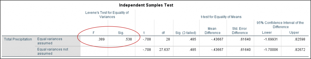
In your Output Viewer window, you should have two tables appear: a general group statistics table with the sample size, mean, standard deviation, and standard error of the mean, and a table with the results of our independent samples test. Note that the “Independent Samples Test” table includes a section labeled “Levene’s Test for Equality of Variances” and two values of the t statistic. Which should we use and what does this test mean? One assumption of the independent samples t-test is the homogeneity of variances, simply meaning that the variance of the samples is roughly equal. In practice, groups with approximately the same size usually have a similar variance, but you could imagine an example where one group is huge and has a high variation in its data and the other is very small and has a relatively low variance. In this case, it would be difficult to make conclusions about the dataset and homogeneity of variance would likely be violated.
Levene’s Test uses the F statistic. In our case, the F statistic is .389 and the significance is .538. The null hypothesis for the Levene’s test is that there is no difference in the variance of the groups tested. Since the significance (or p-value) is greater than .05, we do not reject this hypothesis and can assume homogeneity of variances. If the reported significance was below .05, we would reject this assumption and would need to use the value of t reported in the “Equal variances not assumed” row.
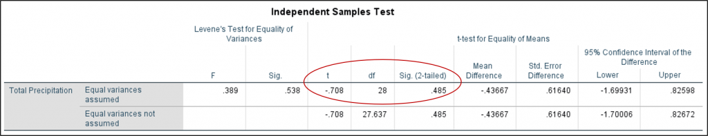
So, since we can assume equal variances, what is the t statistic and the significance? The obtained value of t is -.708 and the significance is .485. This means that while there was slightly less rainfall in rural areas in Florida than urban areas (which you can see in the “Group Statistics” table), the difference was not statistically significant.
What if we compared temperatures rather than rainfall? Re-run the test and switch out “Average Temperatures” for the “Total Precipitation” variable and see if there’s a significant difference. Don’t forget to check for homogeneity of variance using Levene’s test and the F statistic provided.
