19

In this lab, we’re going to learn how conduct a dependent t-test, also known as a paired t-test or repeated measures t-test, using Excel. For this lab, we’ll be exploring global climate data in the “US_Temperatures.xlsx” dataset. This dataset was created by generating a random list of 30 U.S. cities, using randomlists.com/random-us-cities, and then finding the mean annual temperature for each city in 1995 and in 2019 using NOAA’s Climate at a Glance: City Time Series (https://www.ncdc.noaa.gov/cag/). If a city was not listed on NOAA’s website or if the temperature data was incomplete, a nearby city was used.

First, open the dataset using Excel. You’ll notice this dataset has four variables: the city name, the state where the city is located, the mean annual temperature in 1995, and the mean annual temperature in 2019. This data would be appropriate for a dependent t-test because we are exploring the difference between two variables that can each be paired up with the same case. Very often, variables in dependent t-tests are observations at different times as in our example. In other cases, you might have participants that are tested more than once, perhaps to determine the efficacy of a medical treatment, for example.

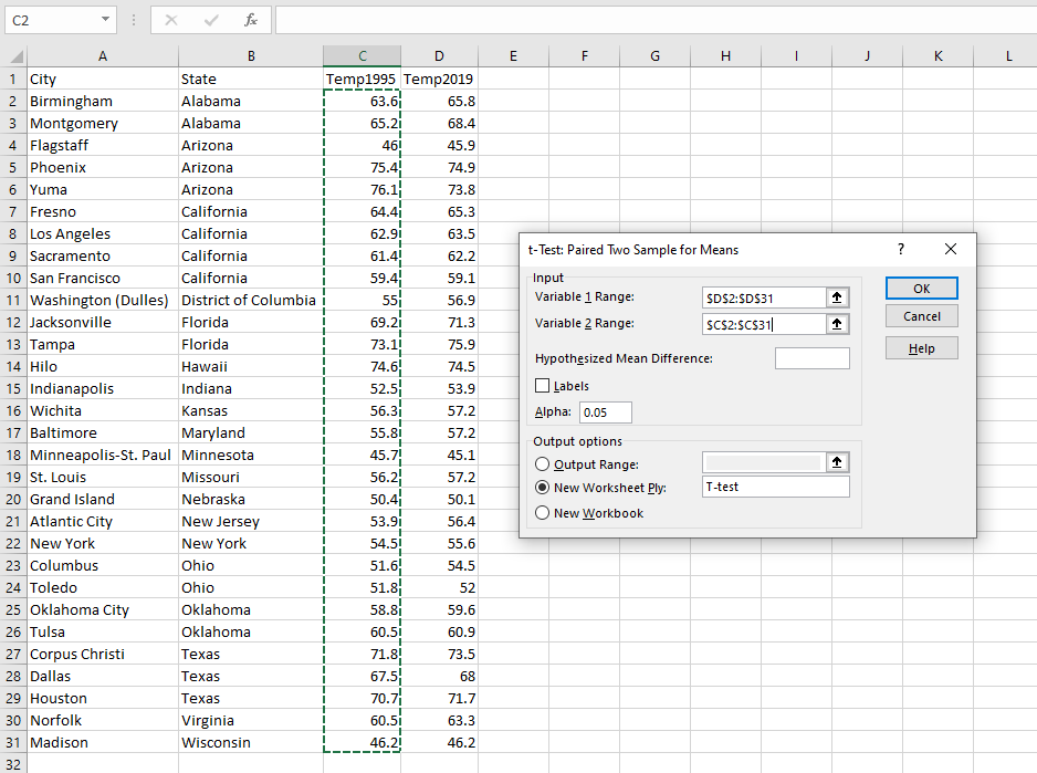
To conduct a dependent samples t-test using Excel, we are going to utilize Excel’s Data Analysis toolpak. Click the Data tab and then click the Data Analysis button. In the dialog box that appears, scroll down and click t-Test: Paired Two Sample for Means. A “paired sample” t-test is another name for a dependent t-test. Then, click OK.

In the window that appears, select the Variable 1 range. Variable 1 should be your “Post” test data. In this case, it would be the temperature in 2019. Select this column of data. For Variable 2, select the temperature in 1995, or the “Pre” test data. Select the button next to “New Worksheet Ply” and create a name for your new worksheet. Then, click OK.

A new worksheet should appear with the results of your t-test. Before proceeding, rename Variable 1 with the appropriate variable name. (In our case, “Temp 2019” or something similar.) Do the same for Variable 2, renaming it “1995”.) If you forget which variables are which, check the values for Mean against the means of each variable in your dataset. Note that Excel presents the “Post” data in the first column.

So how do we interpret these results? Notice that the mean temperature increased slightly from 1995 to 2019. Is this considered a significant increase? What is the value of the t-statistic? You’ll find it labeled “t Stat.” In this case, the value of the t-statistic is approximately 4.22. This, too, supports our conclusion that temperatures increased from our pre-test to post-test. (A negative t-statistic would indicate a decrease, which is also why it is critical to always assign your “Post” variable as Variable 1 and “Pre” variable as Variable 2. Excel subtracts pre- from post- when calculating the t-statistic.)

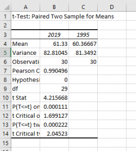
What is the p-value of our test statistic? It is 0.0001.  Is this less than .05? Considerably! This means we have less than a .01% chance of making a Type II error and can conclude that the temperature has significantly increased from 1995 to 2019. You can record the p-value as “p<.01.”