22

This lab will cover both linear regression and multiple regression using SPSS. We will be working with the “Galapagos.sav” dataset, which is a classic example used to teach regression analysis. This data is from M.P. Johnson and P.H. Raven’s 1973 paper: “Species number and endemism: The Galapagos Archipelago revisited” which was published in Science (volume 179, pages 893-895.) Additional elevation data was gathered from http://www.stat.nthu.edu.tw/~swcheng/Teaching/stat5230/data/gala.txt. Regression analysis is commonly utilized by geographers so learning how to use SPSS to compute and analyze a linear regression and multiple regression equation is a valuable skill.

To begin, open the dataset using SPSS. You’ll notice that this dataset has seven variables: the island name, number of species, area (in km squared), elevation (in m), distance to the nearest island (in km), distance to Santa Cruz (located in the center of the Galapagos archipelago), and the area of the adjacent island (in km squared.)

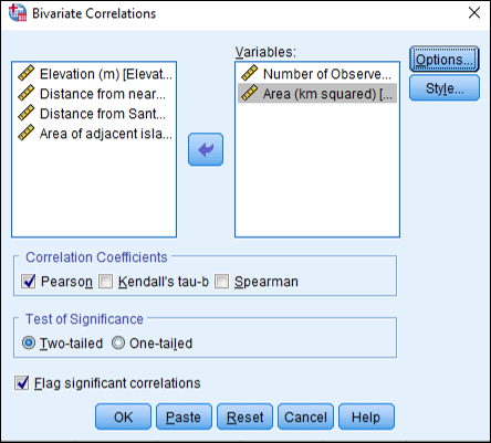
We’re interested in figuring out what is impacting the variety of species found on these islands. We think it might have something to do with the area of the island, so let’s start there. We’ve already learned how to compute the correlation coefficient using SPSS, but now let’s learn how to test it for statistical significance. Click on Analyze, then Correlate, then Bivariate (since we’re beginning by looking at two variables.) Move “Number of Observed Species” and “Area” into the “Variables” box by either clicking the variable and then the arrow or by double-clicking the variables. Be sure there is a check mark next to “Pearson” in the Correlation Coefficients area and also be sure “Flag significant correlations” is checked. Lastly, click OK.

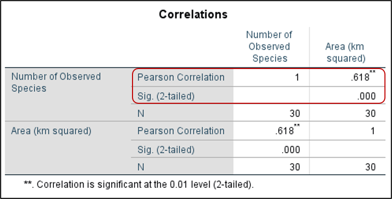
You should now see a Correlations table in your Output Viewer window. What is the correlation between the number of observed species and the size of the island? The correlation coefficient is .618. Using the correlation coefficient rule of thumb, how would you describe this correlation? Is it significant?

So there seems to be a strong relationship between the number of observed species found on an island and the size of the island. What if a new island was discovered and we weren’t sure how many species were found on the island? Could we predict the number of species based on the observed relationship between species number and size? What other variables might impact the number of species found on the island? This is where linear and multiple regression comes in!

To conduct a linear regression analysis using SPSS, click on Analyze, then Regression, then Linear. A “Linear Regression” dialog box should appear. What is our dependent variable? In this case, it’s the number of species because we’re wondering what impacts the number of species found on an island. Move “Number of Observed Species” to the “Dependent” box. What is the independent variable? In this case, it’s area, so move “Area (km squared)” to the “Independent(s)” box. Finally, click OK.

You should see three tables in your Output Viewer window. The first is the “Model Summary.” Notice the value in the R column, which is .618. This number looks familiar… Remember R stands for the correlation coefficient, so it’s the same value we obtained when calculating the correlation coefficient! You’ll also see the R squared value, which in our case is .382, meaning that 38.2% of the variation in the relationship between these two variables is explained by this linear regression model.

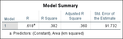
R squared is one way to analyze the accuracy of a linear regression model. We also have the Standard Error of the Estimate, which is a measure of essentially the average error in our model. This is another way to analyze the accuracy of a linear regression model. Our goal is to capture as much of the variation between the variables as we can (maximizing the R squared value) while minimizing the error (reducing the Standard Error of the Estimate.)

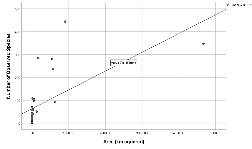
So how could we make a prediction based on our analysis? Notice the “Coefficients” table. Specifically, the “B” column in the “Unstandardized Coefficients” column contains the values needed for our linear regression equation. Remember that a regression equation is written as Y = a + bX, where Y is the dependent variable, X is the independent variable, b is the slope, and a is the intercept. In SPSS, the intercept (a) is found next to “(Constant)” in the column labeled B. The slope (b) is found next to the independent variable also in the “B” column.

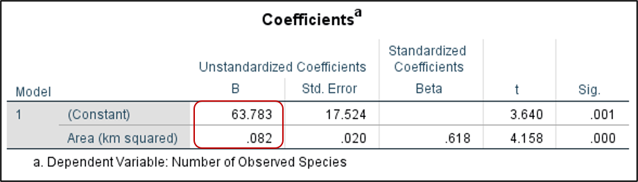
For our example, the equation would be written as Number of Observed Species (Y) = 63.783 + 0.082(Area of the island). So what if our newly discovered island was 100 km squared? How many species would we expect to find? Y = 63.783 + 0.082 (100) which equals 71.983 species.

Another way to explore this data and visualize our regression line is through a scatterplot. Use the instructions in the previous lab on charting and displaying data with SPSS chart builder, or for a quick method of making a scatterplot, click on Graphs, then Legacy Dialogs, then Scatter/Dot. In the Scatter/Dot dialog box that appears, be sure “Simple Scatter” is selected and then click Define. Move “Number of Observed Species” to the “Y Axis” box and move “Area (km squared)” to the “X Axis” box and then click OK. A simple scatterplot should appear in your Output Viewer window. Double click the graph to bring up the “Chart Editor” window. Now, click Elements and then click Fit Line at Total. This will plot a regression line on your scatterplot, while also providing you with the regression equation and the R squared value. This is a good way to double-check that you’ve written your equation correctly.

Well, we now know how to compute a linear regression equation and make predictions, but what if we have other possible independent variables? With multiple regression, we can use multiple independent variables and weight each of them to help make an even more accurate prediction. The steps in conducting a multiple regression in SPSS are the same as for linear regression except that we utilize more independent variables. So, click on Analyze, then Regression, then Linear. Now, though, put all of the other variables in the “Independent(s)” box. Be sure “Number of Observed Species” is in the “Dependent” box. Next to “Method,” you should see the option “Enter” selected. This is the standard regression analysis used by SPSS. Click OK.

You should see similar tables as our previous example in the Output Viewer window. We have a new model summary. What is the new R squared and Standard Error of the Estimate? Has our model improved with the additional variables? We’ve been able to improve our R squared while also reducing our Standard Error. Nice work! This means our multiple regression model is more accurate than the previous linear regression model.

Are all of our variables statistically significant? Check the ANOVA table. Here we see the obtained F statistic and its significance. This tells us whether or not our independent variables have a statistically significant relationship with our dependent variable and whether our model as a whole is a good fit for explaining variation in the number of observed species. In our case, it is since the significance is far below .05.

Now let’s check our “Coefficients” table. Note the values in the “B” column as in the previous linear regression example. Here we find the value of a (or the slope) for each of our independent variables and we also find our intercept.

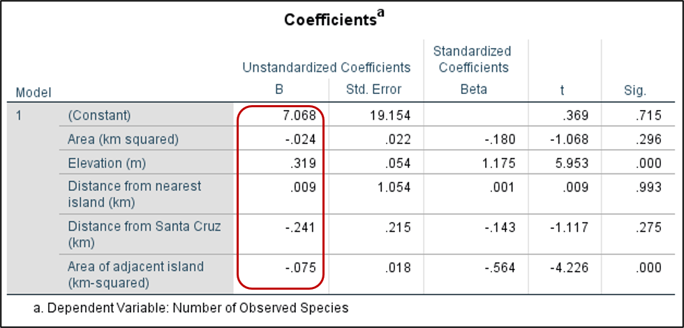
How would we write our multiple regression equation? Number of Observed Species (Y) = 7.068 – 0.024(Area of the island) + 0.319(Elevation) + 0.009(Distance from nearest island) – 0.241(Distance from Santa Cruz) – 0.075(Area of adjacent island). Often, researchers use letters to represent these independent variables and make the equation more streamlined.

Thus, if we discovered a new island and had some basic data on the island, we would be able to estimate, with a relatively high degree of confidence, how many species would likely be found there.

Sometimes we’ll find that our model isn’t statistically significant, or that one independent variable isn’t statistically significant. In these cases, we should re-run the model, removing insignificant or redundant variables. It might take a few tries of running multiple regression models to find a model that fits the data best. Our general goal is to have a statistically significant model with the maximum the R squared value, the minimum the Standard Error of the Estimate, and the simplest model possible. A model with 3 independent variables and a relatively high R squared and low standard error is better than a model with 19 independent variables and a high R squared and low standard error. Play around with your data and see how adding and removing variables impacts the accuracy and error of your model.