UNIT 21 – Electric Field

Beta Keramati

Electrostatics I – Electric Charge, Force, and Field

Last Update: 06/23/2022

the electric field of a point charge

We know electric charges interact with one another without any contact. For example, a positively charged glass rod attracts a negatively charged acrylic rod from a distance. The concept of an electric field helps us explain how the two charged objects can interact without any physical contact.

Consider a point charge that we are going to call a “source charge”, and represent with Q. This source charge creates an electric field around it. You can think of this electric field as being a disturbance in space that surrounds the source charge (hence the name source charge, because this particular point charge is the source of the electric field we are considering). If we bring in another point charge, that we are going to call test charge, and represent with q, and place it in the electric field of the source charge, that test charge is going to experience a force. This is the same Coulomb Force we discussed in UNIT 20. We can think of it this way: the test charge q interacts with the electric field of the source charge, Q, and this interaction manifests itself in the form of a force on the test charge.

the electric field of a point charge

The electric field is a vector quantity. In this section, we discuss how to determine the magnitude and direction of the electric field of a single point charge.

The electric field is defined as the ratio of the Coulomb force to the test charge:

$\boxed{\vec E=\frac{\vec F}{q}}$ Definition of Electric Field

If the electric field is due to a point charge Q, the force on the test charge, calculated by using Coulomb’s law, is given by $F=k\frac{Qq}{r^2}$ . Therefore, the magnitude of the electric field at a point in space in the vicinity of a source charge, Q, is

$\boxed{|\vec E|=k\frac{|Q|}{r^2}}$ Eelectric Field of A Point Charge

In this equation

$Q$ is the source charge creating the electric field $\vec E$ .

$r$ is the distance between the source charge and the point in space where we are calculating the magnitude of the electric field.

$k$ is a constant, called Coulomb’s constant, $k=9.0 \times 10^9 Nm^2/C^2$

The direction of the electric field at that point is the same as the direction of the force that the source charge, Q, would apply on a positive test charge placed at that point. This means that the direction of the electric field around a positive source charge points radially outward, while the electric field of a negative source charge points radially inward.

Figure 21.1 and Figure 21.2 show the electric field vectors at several points around a positive and negative source charge respectively. Notice how the electric field gets weaker at points farther away from the source charge.

You can explore the magnitude and direction of the electric field at various points in space around positive and negative charges using the simulation below.

Rearranging the equation that defines electric field we get

$\vec F=q\vec E$ Force On Charge q Placed In An External Electric Field

This equation is very useful because it means that if we know the electric field at a point in space (whether it is created by one source charge or many source charges), we can determine the force on any charge, q, placed at that point.

One way to represent the electric field around a point charge is with vectors, as demonstrated in Figures 21.1, and figure 21.2. Another way is to draw field lines. Continuous field lines have the same direction at any point as the electric field vector. The closeness of the lines is directly related to the strength of the electric field. Figure 21.3(a) is the vector representation, and Figure 21.3(b) is the field line representation of the electric field around a positive point charge

Since a greater point charge has a stronger electric field around it, we need to draw more field lines to represent that. This is shown in Figure 21.4(b) and (c) for negative point charges.

Example 21.1

A point charge of 2.00nC is placed at the origin of a coordinate system.

a) Calculate the strength and direction of the electric field due to this charge at point P(2.00mm, 4.00mm)

b) What force does the electric field found in (a) exert on a point charge of <span id="MathJax-Element-477-Frame" class="MathJax" style="font-style: normal;font-weight: normal;line-height: normal;font-size: 14px;text-indent: 0px;text-align: left;text-transform: none;letter-spacing: normal;float: none;direction: ltr;max-width: none;max-height: none;min-width: 0px;min-height: 0px;border: 0px;padding: 0px;margin: 0px" role="presentation" data-mathml=" $–0.250 μ C$ “>–0.250μC?

Solution for (a)

Since the source charge is positive, the electric field at point P is a vector pointing away from the source charge, as shown in Figure 21.6.

The magnitude of this electric field is given by

$|\vec E|=k\frac{|Q|}{r^2}$

$|\vec E|=(9.0 \times 10^9 Nm^2/C^2)\frac{2.00 \times 10^{-9}C}{(2.00 \times 10^{-3}m)^2+ (4.00 \times 10^{-3}m)^2}$

$|\vec E|=9.00 \times 10^5 N/C$

We need to find the angle α to specify the direction of the electric field.

$tan\alpha = \frac{4.00mm}{2.00mm}$

$\alpha =63.4^\circ$

The electric field at point P is $\vec E=9.00 \times 10^5 N/C\ @\ 63.4^\circ$

Solution for (b)

There are two ways to answer this question. One way is to use Coulomb’s law ( $|\vec F|=k\frac{|Q| |q|}{r^2}$ ) to calculate the force between the two charges. But since we have already determined the electric field of Q at point P, a much easier way is to use this electric field to find the force on q=<span id="MathJax-Element-477-Frame" class="MathJax" style="font-style: normal;font-weight: normal;line-height: normal;font-size: 14px;text-indent: 0px;text-align: left;text-transform: none;letter-spacing: normal;float: none;direction: ltr;max-width: none;max-height: none;min-width: 0px;min-height: 0px;border: 0px;padding: 0px;margin: 0px" role="presentation" data-mathml=" $–0.250 μ C$ “>–0.250μC.

<span id="MathJax-Element-477-Frame" class="MathJax" style="font-style: normal;font-weight: normal;line-height: normal;font-size: 14px;text-indent: 0px;text-align: left;text-transform: none;letter-spacing: normal;float: none;direction: ltr;max-width: none;max-height: none;min-width: 0px;min-height: 0px;border: 0px;padding: 0px;margin: 0px" role="presentation" data-mathml=" $–0.250 μ C$ “> $\vec F=q\vec E$

Since the charge that is placed in the electric field is negative, the direction of the force on it is opposite to the direction of the electric field, and its magnitude is

<span id="MathJax-Element-477-Frame" class="MathJax" style="font-style: normal;font-weight: normal;line-height: normal;font-size: 14px;text-indent: 0px;text-align: left;text-transform: none;letter-spacing: normal;float: none;direction: ltr;max-width: none;max-height: none;min-width: 0px;min-height: 0px;border: 0px;padding: 0px;margin: 0px" role="presentation" data-mathml=" $–0.250 μ C$ “> $|\vec F|=(-0.250 \times 10^{-6}C)(9.00 \times 10^5 N/C)$

<span id="MathJax-Element-477-Frame" class="MathJax" style="font-style: normal;font-weight: normal;line-height: normal;font-size: 14px;text-indent: 0px;text-align: left;text-transform: none;letter-spacing: normal;float: none;direction: ltr;max-width: none;max-height: none;min-width: 0px;min-height: 0px;border: 0px;padding: 0px;margin: 0px" role="presentation" data-mathml=" $–0.250 μ C$ “> $|\vec F|=0.225N$

To get the direction of this force, we need to find Θ.

$\theta=\alpha + 180^\circ$

$\theta=63.4^\circ+ 180^\circ$

$\theta=243^\circ$

The force on charge q is<span id="MathJax-Element-477-Frame" class="MathJax" style="font-style: normal;font-weight: normal;line-height: normal;font-size: 14px;text-indent: 0px;text-align: left;text-transform: none;letter-spacing: normal;float: none;direction: ltr;max-width: none;max-height: none;min-width: 0px;min-height: 0px;border: 0px;padding: 0px;margin: 0px" role="presentation" data-mathml=" $–0.250 μ C$ “> $\vec F=0.225N\ @\ 243^\circ$

the electric field of multiple point charges

The total electric field created by multiple charges is the vector sum of the individual fields created by each charge. The following example shows how to add electric field vectors.

Example 21.2

Point charge q₁=5.00nC is at (0, – 2.00cm), and point charge q₂ = 10.0nC is at (4.00cm, 0). Find the magnitude and direction of the total electric field due to the two point-charges at the origin of the coordinate system.

Solution

We need to find the electric field due to each charge separately, and then add the two vectors together to get the total electric field.

The electric field due to q₁ is

$|\vec E_1|=k\frac{q_1}{r_1^2}$

$|\vec E_1|=(9.0 \times 10^9 Nm^2/C^2)\frac{5.00 \times 10^{-9}C}{(2.00 \times 10^{-2}m)^2}$

$|\vec E_1|=1.125 \times 10^5 N/C$

The electric field due to q₂ is

$|\vec E_2|=k\frac{q_2}{r_2^2}$

$|\vec E_2|=(9.0 \times 10^9 Nm^2/C^2)\frac{10.0 \times 10^{-9}C}{(4.00 \times 10^{-2}m)^2}$

$|\vec E_1|=5.625 \times 10^4 N/C$

Now we have to add the two vectors

$\vec E_1= 0 \hat i +1.125 \times 10^5 N/C \hat j$

$\vec E_2= 5.625 \times 10^4 N/C \hat i +0 \hat j$

We can leave the answer in component form as following:

$\vec E_{tot}=\vec E_1 +\vec E_2= 5.625 \times 10^4 N/C \hat i +1.125 \times 10^5 N/C \hat j$

Or, we can find magnitude and direction of $\vec E_{tot}$

$|\vec E_{tot}|=\sqrt{ (5.625 \times 10^4 N/C)^2 + (1.125 \times 10^5 N/C)^2}$

$|\vec E_{tot}|=1.26 \times 10^5 N/C$

Let’s call the angle $\vec E_{tot}$ makes with the negative x axis Θ.

$tan\theta=\frac{1.125 \times 10^5 N/C}{5.625 \times 10^4 N/C}$

$\theta=63.4^\circ$

So the angle relative to positive x axis is

$180^\circ-63.4^\circ=117^\circ$

Therefore, in terms of magnitude and direction, $\vec E_{tot}$ is

$\vec E_{tot}=1.26 \times 10^5 N/C\ @\ 117^\circ$

Figure 21.9 shows how the electric field from two point-charges can be drawn by finding the total field at representative points and drawing electric field lines consistent with those points. While the electric fields from multiple charges are more complex than those of single charges, some simple features are easily noticed.

For example, the field is weaker between like charges, as shown by the lines being farther apart in that region. This is because the fields from each charge exert opposing forces on any charge placed between them. See Figure 21.10(a) and (b). Furthermore, at a great distance from two like charges, the field becomes identical to the field from a single, larger charge.

We use electric field lines to visualize and analyze electric fields (the lines are a pictorial tool, not a physical entity in themselves). The properties of electric field lines for any charge distribution can be summarized as follows:

Field lines must begin on positive charges and terminate on negative charges, or at infinity in the hypothetical case of isolated charges.
The number of field lines leaving a positive charge or entering a negative charge is proportional to the magnitude of the charge.
The strength of the field is proportional to the closeness of the field lines—more precisely, it is proportional to the number of lines per unit area perpendicular to the lines.
The direction of the electric field is tangent to the field line at any point in space.
Field lines can never cross.

The last property means that the field is unique at any point. The field line represents the direction of the field; so if they crossed, the field would have two directions at that location (an impossibility if the field is unique).

Applications of electric field

Gel Electrcophoresis

DNA is a highly charged molecule. It is the electrostatic force that not only holds the molecule together but gives the molecule structure and strength.Figure 21.11 is a schematic of the DNA double helix.

Gel electrophoresis is a technique used to separate DNA fragments of different sizes. The DNA is loaded on the gel and an electric current is applied. The DNA has a net negative charge and moves from the negative electrode toward the positive electrode. The electric current is applied for sufficient time to let the DNA separate according to size; the smallest fragments will be farthest from the well (where the DNA was loaded), and the heavier molecular weight fragments will be closest to the well. Once the DNA is separated, the gel is stained with a DNA-specific dye for viewing it.

Xerography

Most copy machines use an electrostatic process called xerography—a word coined from the Greek words xeros for dry and graphos for writing. The heart of the process is shown in simplified form below.

A selenium-coated aluminum drum is sprayed with a positive charge from points on a device called a corotron. Selenium is a substance with an interesting property—it is a photoconductor. That is, selenium is an insulator when in the dark and a conductor when exposed to light.

In the first stage of the xerography process, the conducting aluminum drum is grounded so that a negative charge is induced under the thin layer of uniformly positively charged selenium. In the second stage, the surface of the drum is exposed to the image of whatever is to be copied. Where the image is light, the selenium becomes conducting, and the positive charge is neutralized. In dark areas, the positive charge remains, and so the image has been transferred to the drum.

The third stage takes a dry black powder, called toner, and sprays it with a negative charge so that it will be attracted to the positive regions of the drum. Next, a blank piece of paper is given a greater positive charge than on the drum so that it will pull the toner from the drum. Finally, the paper and electrostatically held toner are passed through heated pressure rollers, which melt and permanently adhere the toner within the fibers of the paper.

Laser Printers

Laser printers use the xerographic process to make high-quality images on paper, employing a laser to produce an image on the photoconducting drum as shown below. In its most common application, the laser printer receives output from a computer, and it can achieve high-quality output because of the precision with which laser light can be controlled. Many laser printers do significant information processing, such as making sophisticated letters or fonts, and may contain a computer more powerful than the one giving them the raw data to be printed.

Ink Jet Printers and Electrostatic Painting

The inkjet printer, commonly used to print computer-generated text and graphics, also employs electrostatics. A nozzle makes a fine spray of tiny ink droplets, which are then given an electrostatic charge.

Once charged, the droplets can be directed, using pairs of charged plates, with great precision to form letters and images on paper. Inkjet printers can produce color images by using a black jet and three other jets with primary colors, usually cyan, magenta, and yellow, much as a color television produces color. (This is more difficult with xerography, requiring multiple drums and toners.)

Smoke Precipitators and Electrostatic Air Cleaning

Another important application of electrostatics is found in air cleaners, both large and small. The electrostatic part of the process places an excess (usually positive) charge on smoke, dust, pollen, and other particles in the air and then passes the air through an oppositely charged grid that attracts and retains the charged particles.

Large electrostatic precipitators are used industrially to remove over 99% of the particles from stack gas emissions associated with the burning of coal and oil. Home precipitators, often in conjunction with the home heating and air conditioning system, are very effective in removing polluting particles, irritants, and allergens.

Attribution

This chapter contains material taken from Openstax College Physics-Electric Charge and Electric Field, and is used under a CC BY 4.0 license. Download these books for free at Openstax

To see what was changed, refer to the List of Changes.

problems

[openstax univ. phys. vol.2 – 5.65] A particle of charge 2.00×10^-8C experiences an upward force of magnitude 4.00×10^-6N when it is placed at a particular point in an electric field.
1. What is the electric field at that point?
2. If a charge q=-1.00×10^-8C is placed there, what is the force on it?
[openstax univ. phys. vol. 2 – 5.67 – modified] Consider an electron that is 1.00×10^-10m to the left of an alpha particle as shown. An alpha particle consists of two protons and two neutrons that are tightly bound together. Therefore, the electric charge of an alpha particle is 3.20×10^-19C).
1. What is the electric field due to the alpha particle at the location of the electron? Draw a vector to show this electric field and label it as $\vec E_{of \alpha particle}$ .
2. What is the electric field due to the electron at the location of the alpha particle? Draw a vector to show this electric field and label it as $\vec E_{of electron}$ .
3. What is the electric force on the alpha particle? Show this force with a vector labeled as $\vec F_{on \alpha particle}$ .
4. What is the electric force on the electron? Show this force with a vector labeled as $\vec F_{on electron}$ .
[openstax univ. phys. vol. 2 – 5.72] A small piece of cork whose mass is 2.00 g is given a charge of5.00×10^-7C. What electric field is needed to place the cork in equilibrium under the combined electric and gravitational forces?
[openstax univ. phys. vol. 2 – 2.73] If the electric field of a point charge q is 100N/C at a distance of 50.0 cm from it. What is the value of q?
[openstax univ. phys. vol. 2 – 5.76 – modified] Two point charges, q₁=2.00×10^-7C and q₂=-6.00×10^-8C are held 25.0 cm apart, with q₁ to the left of q₂.
1. What is the magnitude and direction of the electric field at a point between the two charges and 5.00 cm from q₁?
2. What is the magnitude and direction of the force on an electron placed at that point?
[openstax univ. phys. vol.2 – 5.79] Point charges q₁=q₂=4.00×10^-6C are fixed on the x-axis at x=-3.00m and x=3.00m. What charge q must be placed at the origin so that the electric field vanishes at x=0, y=3.00m?
[openstax unv. phys. vol. 2 – 5.91] A proton moves in the electric field
1. Determine the force on the proton and its acceleration?
2. Do the same calculation for an electron moving in this field.
[openstax univ. phys. vol. 2 – 5.92] An electron and a proton, each starting from rest, are accelerated by the same uniform electric field of 200 N/C. Determine the distance and time for each particle to acquire kinetic energy of 3.20×10^-16J.
[openstax univ. phys. vol. 2 – 5.93] A spherical water droplet of radius 25.0μm carries an excess of 250 electrons. What vertical electric field (magnitude and direction) is needed to balance the gravitational force on the droplet?
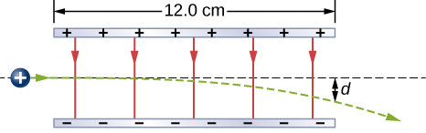
[openstax univ. phys. vol. 2 – 5.94] A proton enters the uniform electric field produced by the two charged plates shown below. The magnitude of the electric field is 4.00×10⁵ N/C, and the speed of the proton when it enters is 1.50×10⁷m/s. What distance d has the proton been deflected downward when it leaves the plates?
[openstax college phys. 18.60] A 5.00 g charged insulating ball hangs on a 30.0 cm long string in a uniform horizontal electric field as shown below. Given the charge on the ball is 1.00μC, find the strength of the field.
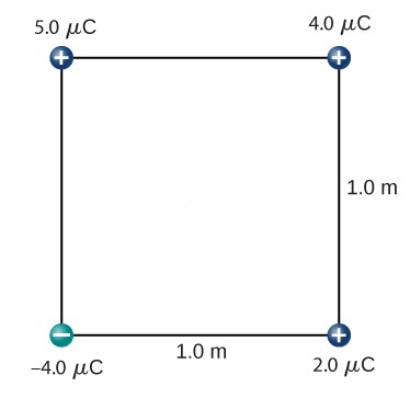
Four point-charges are held at the corners of a square as shown.
1. Determine the magnitude and direction of the electric field in the center of the square.
2. Determine the magnitude and direction of the force experienced by a 2.00µC charge placed at the center of the square.
3. Determine the magnitude and direction of the force experienced by a -2.00µC charge placed at the center of the square.