UNIT 22 – Electric Potential Energy, and Electric Potential

Beta Keramati

Electrostatics II – Electric Potential, and Capacitors

Last Update: 06/24/2022

electric potential energy

The electrostatic or Coulomb force is conservative. This means that when negative work done by the Coulomb force removes kinetic energy from the system, that energy is stored in the form of electric potential energy, and can be converted back into kinetic energy again when the Coulomb force does positive work. (For a review of conservative forces and their relationship to potential energy, see UNIT 11.) We can express this with the following equation.

$W_{Coulomb\ force}=-\Delta U_{electric}$

Let’s consider a uniform electric field. By “uniform” we mean an electric field that is constant everywhere, as shown in Figure 22.1.

Suppose a point charge, q has a displacement, d, in this electric field. Since the electric field is constant, the force on this charge is also constant. As discussed in UNIT 10, work done by a constant force is $W=Fdcos\theta$ . Therefore

$W=-\Delta U=qEdcos\theta$ In A Constant Electric Field

When a positive charge moves in the direction of the field, its potential energy decreases, and if it moves opposite to the direction of the field, its potential energy increases. The opposite is true for a negative charge. In other words, if a point charge is released in an electric field, it moves in a direction that would decrease its electric potential energy. Just like when an object is released close to the surface of the earth, it moves in a direction that would decrease its gravitational potential energy, which is straight down.

electric potential

Electric potential is defined as electric potential energy per unit charge. Electric potential is represented with V and is measured in Joule/Coulomb which is known as volt.

$\boxed{V=\frac{U_{electric}}{q}}$ Electric potential

Example 22.1

You have a 12.0-V motorcycle battery that can move 5000 C of charge, and a 12.0-V car battery that can move 60,000 C of charge. How much energy does each deliver? (Assume that the numerical value of each charge is accurate to three significant figures.)

Solution

We need to determine by how much the electric potential energy of the given charge changes when it moves through a difference in potential of 12.0V. Since electric potential and electric potential energy are related according to $V=\frac{U_{electric}}{q}$ , we can conclude that

$\Delta V=\frac{\Delta U_{electric}}{q}$

For the motorcycle battery we get

$12.0V=\frac{\Delta U_{electric}}{5000C}$

$\Delta U=6.00 \times 10^4 J$

For the car battery we get

$12.0V=\frac{\Delta U_{electric}}{60,000C}$

$\Delta U=7.20 \times 10^5 J$

Discussion

Voltage and energy are related, but they are not the same thing. The voltages of the batteries are identical, but the energy supplied by each is quite different. Using the analogy with gravity, this is like a bowling ball and a ping pong ball starting side by side at the top of a hill and rolling down. The bowling ball has a lot more energy at the bottom of the hill compared to the ping pong ball, even though both balls went through the same change in elevation. Just like the greater mass of the bowling ball accounts for more energy at the bottom of the hill, the greater charge that is being moved in a car battery accounts for greater energy delivered by the battery.

Electric potential is a property of space. A charge creates an electric potential around it. When another charge is brought nearby, the system of two charges has electric potential energy. This is somewhat similar to the difference between electric field and electric force. A single charge (a source charge) creates an electric field around it. When another charge (a test charge) is placed in that electric field, the system of two charges interact and the interaction manifests itself in the form of a force between the two charges.

Using the analogy with gravity, we can think of the electric potential in an electric field as elevation in a gravitational field. But since there are two types of charges, positive, and negative, the electric potential around a positive charge is positive (above zero), while the electric potential around a negative charge is negative (below zero). The electric potential around positive and negative point charges can be visualized as depicted in Figure 22.2. Imagine the positive charge that is creating this potential to be at the top of the infinitely tall mountain on the left and the negative point charge at the bottom of the infinitely deep hole on the right. Where the surface is flat, the electric potential is zero.

Using calculus it can be shown that the electric potential around a point charge, Q, is given by

$\boxed{V=k\frac{Q}{r}}$ Electric Potential Of A Point Charge

Electric potential is a scalar quantity but it can be positive or negative depending on the charge. Notice that the electric potential of a point charge is zero at a distance infinitely far away from the point charge (when r→∞). This is consistent with the visualization in Figure 22.2 where the flat surface represents V=0, and this surface is infinitely far away from the top of the infinitely tall mountain that represents the positive charge, or the bottom of the infinitely deep hole that represents the negative charge.

If two point-charges, q₁ and q₂, are held next to one another, the two charges either repel or attract each other. So if they are held in place next to one another, the system of the two charges has a certain amount of potential energy. We can determine the potential energy of the system by combining $V=\frac{U_{electric}}{q}$ , and $V=k\frac{Q}{r}$ . The result is

$\boxed{U_{electric}=k\frac{q_1 q_2}{r}}$ Potential Energy of Two Point Charges

Example 22.2

Find the amount of work an external agent must do in assembling four charges +2.0μC, +3.0μC, +4.0μC, and, +5.0μC at the vertices of a square of side 1.0 cm, starting each charge from very far away.

Solution

We bring in the charges one at a time and calculate the work to bring them in from very far away to their final location.

First, bring the +2.0μC charge. Since there are no other charges at a finite distance from this charge yet, no work is done in bringing it from very far away.

$W_1=0$

While keeping the +2.0μC charge fixed at one corner of the square, we bring the +3.0μC charge to its place. Now, the applied force must do work against the force exerted by the +2.0μC charge fixed in its place. The work done equals the change in the potential energy of the +3.0μC.

$W_2 = k\frac{q_1 q_2}{r_{12}}$

$W_2 = (9.0\times 10^9) \frac{N}{m^2C^2}\frac{(+2.0 \times 10^{-6} C)(+3.0 \times 10^{-6} C)}{0.010m}$

$W_2 = 5.4J$

While keeping the charges of 2.0μC and 3.0μC fixed in their places, bring in the 4.0μC charge and place it at another corner of the square. The work done in this step increases the potential energy of the 4.0μC charge.

$W_3 = k\frac{q_1 q_3}{r_{13}}+k\frac{q_2 q_3}{r_{23}}$

$W_3 = (9.0\times 10^9 \frac{N}{m^2C^2})\frac{(+2.0 \times 10^{-6} C)(+4.0 \times 10^{-6}C)}{\sqrt{(0.010m)^2+(0.010m)^2}}+ (9.0\times 10^9 \frac{N}{m^2C^2})\frac{(+3.0 \times 10^{-6} C)(+4.0 \times 10^{-6} C)}{0.010m}$

$W_3= 15.9J$

Finally, while keeping the first three charges in their places, we bring the 5.0μC charge and place it on the last corner of the square. Once again, the work done is equal to the increase in the potential energy of the 5.0μC charge.

$W_4 = k\frac{q_1 q_4}{r_{14}}+k\frac{q_2 q_4}{r_{24}} + k\frac{q_3 q_4}{r_{34}}$

$W_3 = (9.0\times 10^9 \frac{N}{m^2C^2})\frac{(+2.0 \times 10^{-6} C)(+5.0 \times 10^{-6}C)}{0.01m}+ (9.0\times 10^9 \frac{N}{m^2C^2})\frac{(+3.0 \times 10^{-6} C)(+5.0 \times 10^{-6} C)}{\sqrt{(0.010m)^2+(0.010m)^2}}+ (9.0\times 10^9 \frac{N}{m^2C^2})\frac{(+4.0 \times 10^{-6} C)(+5.0 \times 10^{-6}C)}{0.01m}$

$W_4= 36.5J$

Therefore, the total work done to assemble the charges on the four corners of the square is

$W_{total}=0+5.4J+15.9J+36.5J$

$W_{total}=58J$

Discussion:

Notice that as more charges are assembled on the corners of the square, more work is needed to bring the next charge in. This makes sense because all the charges are positive and they repel each other.

Also, the work on each charge depends only on its pairwise interactions with the other charges. No more complicated interactions need to be considered; the work on the third charge only depends on its interaction with the first and second charges, the interaction between the first and second charges does not affect the third.

Once again, using the analogy with gravity and the visualization depicted in Figure 22.2, we can think of the difference in potential between two points to be like a difference in elevation. The difference in electric potential between two points is known as voltage.

Visualizing electric potential as shown in Figure 22.2, we can see that when a positive charge is released in a region where there is a difference in potential, the positive charge moves from high to low potential (downhill), whereas a negative charge moves from low to high potential (uphill).

Furthermore, since the direction of the electric field is always from positive charge to negative charge, in terms of electric potential, the electric field always points from high potential to low potential.

Example 22.3

Calculate the final speed of a free electron accelerated from rest through a voltage (potential difference) of 100 V.

Solution

The electric force is a conservative force. Therefore, as the electron accelerates, the mechanical energy is conserved. We can use the relationship between electric potential and potential energy to find the change in potential energy. The charge of an electron is -1.60×10^-19C. For the electron to speed up, it has to move from low to high potential. Therefore ΔV>0.

$\Delta V=\frac{\Delta U_{electric}}{q}$

$100V=\frac{\Delta U}{-1.60 \times 10^{-19}C}$

$\Delta U=-1.60 \times 10^{-17}J$

Now we use conservation of mechanical energy to find the change in kinetic energy and from that determine the final speed.

$\Delta KE + \Delta U=0$

$\Delta KE - 1.60 \times 10^{-17}J=0$

$\Delta KE =1.60 \times 10^{-17}J$

Mass of an electron is 9.11×10^-31kg.

$\frac{1}{2}(9.11 \times 10^{-31}kg)v^2-0=1.60 \times 10^{-17}J$

$v=5.93\times 10^6 m/s$

Discussion

In this problem, we ignored the gravitational force on the electron. In general, when dealing with subatomic particles in electric fields, the gravitational force on the particle is almost always negligible.

Example 22.4

Consider the dipole in Figure 22.2.1 with the charge magnitude of q=3.0nC and separation distance d=4.0cm. What is the potential at the following locations in space? (a) (0, 0, 1.0 cm); (b) (0, 0, –5.0 cm); (c) (3.0 cm, 0, 2.0 cm).

Solution for a

We need to calculate the electric potential due to each charge and add them together. Electric potential is a scalar quantity, so there is no direction to worry about, but we have to keep track of signs.

$V=k\frac{Q_1}{r_1} +k\frac{Q_2}{r_2}$

$V=(9.0 \times 10^9 Nm^2/C^2)\frac{+3.0 \times 10^{-9}C}{0.010m} +(9.0 \times 10^9 Nm^2/C^2)\frac{-3.0 \times 10^{-9}C}{0.030m}$

$V=1.8 \times 10^3 V$

Solution for b

Using the same process we get

$V=k\frac{Q_1}{r_1} +k\frac{Q_2}{r_2}$

$V=(9.0 \times 10^9 Nm^2/C^2)\frac{+3.0 \times 10^{-9}C}{0.070m} +(9.0 \times 10^9 Nm^2/C^2)\frac{-3.0 \times 10^{-9}C}{0.030m}$

$V=-5.1 \times 10^2 V$

Solution for c

We use Pythagorean Theorem to find the distance between the negative charge and the point at which we want to find the potential.

$r_2=\sqrt{(0.040m)^2+(0.030m)^2}$

$r_2=0.050m$

$V=k\frac{Q_1}{r_1} +k\frac{Q_2}{r_2}$

$V=(9.0 \times 10^9 Nm^2/C^2)\frac{+3.0 \times 10^{-9}C}{0.030m} +(9.0 \times 10^9 Nm^2/C^2)\frac{-3.0 \times 10^{-9}C}{0.050m}$

$V=3.6 \times 10^2 V$

In a constant electric field, we can easily find a relationship between voltage (difference in electric potential) and electric field by using the relationship between work and change in potential energy. As mentioned earlier, in a constant electric field

$W=-\Delta U=qEdCos\theta$

Dividing by q yields

$\boxed{|\Delta V|=|EdCos\theta|}$ In A Constant Electric Field

In this equation

$\Delta V$ is the difference in potential between two points.

$E$ is the constant electric field in the region.

$d$ is the distance between the two points.

$\theta$ is the angle between $d$ and $E$

To get the signs right, we need to remember that the electric field always points from high potential to low potential.

Example 22.5

Dry air can support a maximum electric field strength of about 3.0×10⁶V/m. Above that value, the field creates enough ionization in the air to make the air a conductor. This allows a discharge or spark that reduces the field. What, then, is the maximum voltage between two parallel conducting plates separated by 2.5 cm of dry air?

Solution

We are given the maximum electric field E between the plates and the distance d between them. We can use the equation $|\Delta V|=|EdCos\theta|$ to calculate the maximum voltage. In this case θ=0 and Cosθ=1.

$|\Delta V|=|Ed|$

$|\Delta V|=|(3.0\times 10^6 Vm)(0.025m)|$

$|\Delta V|=7.5\times 10^4 V$

Discussion

One of the implications of this result is that it takes about 75 kV to make a spark jump across a 2.5-cm (1-in.) gap, or 150 kV for a 5-cm spark. This limits the voltages that can exist between conductors, perhaps on a power transmission line. A smaller voltage can cause a spark if there are spines on the surface since sharp points have larger field strengths than smooth surfaces. Humid air breaks down at a lower field strength, meaning that a smaller voltage will make a spark jump through the humid air. The largest voltages can be built up with static electricity on dry days.

Equipotential lines and surfaces

In a two-dimensional situation, an equipotential line is a line that consists of points that are at the same electric potential. Similarly, for a three-dimensional configuration, an equipotential surface is a surface where all the points are at the same electric potential. Mapping equipotential lines on a two-dimensional surface is a lot like creating a topographic map to show points that are at the same elevation. Consider the following topographic map.

On this map, a line is drawn for every 20ft of change in elevation. Therefore, the areas where the lines are close to one another represent a steep terrain, while where the lines are farther apart shows a more flat region. The same idea is represented in the topographic map of Devils Tower, also known as Bear Lodge, in Wyoming.

Let’s create a similar plot for equipotentials around a point charge. Since the electric potential of a point charge is given by $V=k\frac{Q}{r}$ all the points that are the same distance away from the point charge are at the same potential. This means equipotential lines are circular, as shown in Figure 22.4.

The circles show the equipotential lines, and the arrows are the electric field lines.

Figure 22.5 (a) shows a few equipotential lines around two negative charges. Figure 22.5(b) also includes the electric field lines in this region.

Figure 22.6 and Figure 22.7 show the equipotential lines around a dipole (a positive and a negative point charge with equal magnitude).

Figure 22.8 and Figure 22.9 show the equipotential lines where the electric field is constant(uniform). In both figures, the lines are equipotential lines, and the arrows are electric field lines.

In the previous section, we showed that the voltage between two points in a uniform electric field is $|\Delta V|=|EdCos\theta|$ . Notice that in a constant electric field, $dCos\theta$ is just the distance between the initial and final equipotential lines, which is the distance between the two green lines, marked as L in Figure 22.10.

We can simplify the result as

$\boxed{|\Delta V|=EL\ ,\ E=\frac{\Delta V}{L}}$ In A Constant Electric Field

where L is the distance between the two equipotential lines.

Up to now, we have been using the units of N/C for the electric field. As evident in the equation above, another standard unit for electric field is volt/meter (V/m).

$1N/C=1V/m$

Notice that regardless of the details of the charge distribution and the shape of equipotential lines, electric field lines are always perpendicular to equipotential lines and they point from high potential to low potential. If the equipotential lines are drawn the same voltage apart, where they are denser, the electric field is stronger, and if they are equal distance apart, the electric field is constant.

It is insightful to think of the electric field as being measured in V/m because it indicates how dense the equipotential lines are in a given region in space.

How Skeletal Muscles Contract

All living cells have membrane potentials or electrical gradients across their membranes. The inside of the membrane is usually around -60 to -90 mV, relative to the outside. This is referred to as a cell’s membrane potential. Neurons and muscle cells can use their membrane potentials to generate electrical signals. They do this by controlling the movement of charged particles, called ions, across their membranes to create electrical currents. This is achieved by opening and closing specialized proteins in the membrane called ion channels. Although the currents generated by ions moving through these channel proteins are very small, they form the basis of both neural signaling and muscle contraction.

Both neurons and skeletal muscle cells are electrically excitable, meaning that they are able to generate action potentials. An action potential is a special type of electrical signal that can travel along a cell membrane as a wave. This allows a signal to be transmitted quickly and faithfully over long distances.

For a skeletal muscle fiber to contract, its membrane must first be “excited”—in other words, it must be stimulated to fire an action potential. The muscle fiber action potential, which sweeps along the sarcolemma as a wave, is “coupled” to the actual contraction through the release of calcium ions (Ca⁺⁺) from the SR (sarcoplasmic reticulum) . Once released, the Ca⁺⁺ interacts with the shielding proteins, forcing them to move aside so that the actin-binding sites are available for attachment by myosin heads. The myosin then pulls the actin filaments toward the center, shortening the muscle fiber. See the video below for an excellent illustration of how all this happens.

Attribution

This chapter contains material taken from Openstax University Physics Volume 2-Electric Potential and is used under a CC BY 4.0 license. Download these books for free at Openstax

The section on How Skeletal Muscles Contract is taken from Anatomy and Physiology-Openstax. Access this book for free at https://openstax.org/books/anatomy-and-physiology/pages/1-introduction

To see what was changed, refer to the List of Changes.

problems

[openstax univ. phys. vol.2 – 7.31-modified] To form a hydrogen atom, a proton is fixed at a point and an electron is brought from far away to a distance of 0.529×10^-10m, the average distance between proton and electron in a hydrogen atom.
1. What is the electric potential at a distance of 0.529×10^-10m from the proton?
2. How much work is done to bring an electron from far away and place it at that point?
[openstax college phys – 19.19] Membrane walls of living cells have surprisingly large electric fields across them due to the separation of ions. What is the voltage across an 8.00 nm–thick membrane if the electric field strength across it is 5.50 MV/m? You may assume a uniform electric field.
[openstax univ. phys. vol. 2 – 7.36] What is the strength of the electric field between two parallel conducting plates separated by 1.00 cm with a potential difference (voltage) of 1.50×10⁴V?
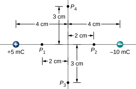
[openstax univ. phys. vol.2 – 7.52] Find the potential at points P₁, P₂, P₃, and P₄ in the diagram due to the two given charges. Assume three significant figures for all the given values.
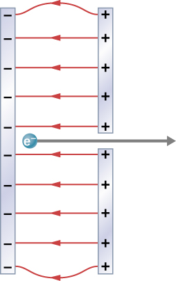
[openstax univ. phys. vol. 2 – 7.70] A simple and common technique for accelerating electrons is shown below, where there is a uniform electric field between two plates. Electrons are released, usually from a hot filament, near the negative plate, and there is a small hole in the positive plate that allows the electrons to continue moving.
1. Calculate the acceleration of the electron if the electric field is 2.50×10⁴N/C.
2. Explain why the electron will not be pulled back to the positive plate once it moves through the hole.
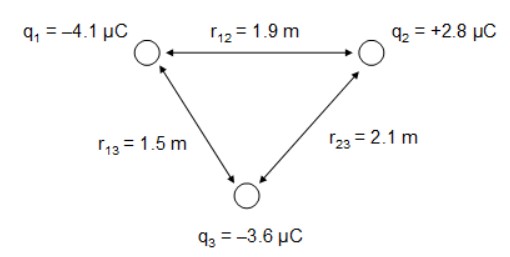
Find the electric potential energy of the charge configuration shown.
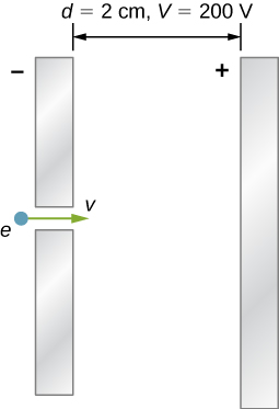
[openstax univ. phys. vol. 2 – 7.77] An electron enters a region between two large parallel plates made of aluminum separated by a distance of 2.00 cm and kept at a potential difference of 200 V. The electron enters through a small hole in the negative plate and moves toward the positive plate. At the time the electron is near the negative plate, its speed is 4.00×10⁵m/s. Assume the electric field between the plates to be uniform. Find the speed of the electron immediately before it hits the positive plate.
[openstax univ. phys. vol. 2 – 7.79]Dry air becomes ionized in an electric field with a strength of 3.00×10⁶V/m.
1. Will the electric field strength between two parallel conducting plates exceed the breakdown strength of dry air if the plates are separated by 2.00 mm and a potential difference of 5.00×10³V is applied?
2. How close together can the plates be with this applied voltage without ionizing the air in between?
The electric field lines in a region in space are shown. The dashed lines are equipotential lines.
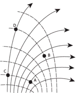
1. Rank the points in terms of electric potential, from highest to lowest.
2. Does the potential energy of a point charge increase, decrease, or remain the same when it is moved from B to C if the point charge is positive? if it is negative?
The figure shows the equipotential lines in a region of space.
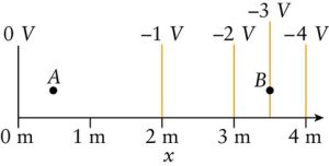
1. Compare the strength of the electric field at points A and B.
2. What is the direction of the electric field in this region?
3. How much work is done to move a +2.00µC charge from -1V to -3V? Is this work done by the force of the electric field or against the force of the electric field? How would your answers change if the charge was -2.00µC?