Unit 3 – Motion with Constant Acceleration

Beta Keramati

Kinematics – Linear Motion

Last Update: 5/10/2024

Acceleration

In everyday conversation, to accelerate means to speed up. The accelerator in a car can in fact cause it to speed up. The greater the acceleration, the greater the change in velocity over a given time. The formal definition of acceleration is consistent with these notions but more inclusive.

average Acceleration

Average Acceleration is the rate at which velocity changes,

$\boxed{\bar{a}=\frac{\Delta v}{\Delta t} = \frac{v - v_0}{t - t_0}}$

where $\bar{a}$ is average acceleration.

Because acceleration is the velocity in m/s divided by time in s, the SI units for acceleration are m/s/s which can also be written as m/s². Meters per second squared or meters per second per second literally means by how many meters per second the velocity changes every second.

Recall that velocity is a vector—it has both magnitude and direction. This means that a change in velocity can be a change in magnitude (or speed), but it can also be a change in direction. For example, if a car turns a corner at a constant speed, it is accelerating because its direction is changing. The quicker you turn, the greater the acceleration. So there is an acceleration when velocity changes either in magnitude (an increase or decrease in speed) or in direction, or both.

Acceleration is a vector in the same direction as the change in velocity.

Keep in mind that although acceleration is in the direction of the change in velocity, it is not always in the direction of motion. When an object slows down, its acceleration is opposite to the direction of its motion. This is known as deceleration.

Deceleration always refers to acceleration in the direction opposite to the direction of the velocity. Deceleration always reduces speed. Negative acceleration, however, is acceleration in the negative direction in the chosen coordinate system. Negative acceleration may or may not be deceleration, and deceleration may or may not be considered negative acceleration. For example, consider Figure 3.1. In (a), the car is speeding up as it moves toward the right. It, therefore, has positive acceleration in our coordinate system. In (b), the car is slowing down as it moves toward the right. Therefore, it has a negative acceleration in our coordinate system because its acceleration is toward the left. The car is also decelerating: the direction of its acceleration is opposite to its direction of motion. In (c), the car is moving toward the left, but slowing down over time. Therefore, its acceleration is positive in our coordinate system because it is toward the right. However, the car is decelerating because its acceleration is opposite to its motion. In (d), the car is speeding up as it moves toward the left. It has a negative acceleration because it is accelerating toward the left. However, because its acceleration is in the same direction as its motion, it is speeding up (not decelerating).

Four separate diagrams of cars moving. Diagram a: A car moving toward the right. A velocity vector arrow points toward the right. An acceleration vector arrow also points toward the right. Diagram b: A car moving toward the right in the positive x direction. A velocity vector arrow points toward the right. An acceleration vector arrow points toward the left. Diagram c: A car moving toward the left. A velocity vector arrow points toward the left. An acceleration vector arrow points toward the right. Diagram d: A car moving toward the left. A velocity vector arrow points toward the left. An acceleration vector arrow also points toward the left. — Figure 3.1

Example 3.1-Calculating Average Acceleration: A Racehorse Leaves the Gate

A racehorse coming out of the gate accelerates from rest to a velocity of 15.0 m/s due west in 1.80 s. What is its average acceleration?

Strategy

First we draw a sketch and assign a coordinate system to the problem. This is a simple problem, but it always helps to visualize it. Notice that we assign east as positive and west as negative. Thus, in this case, we have negative velocity.

An acceleration vector arrow pointing west, in the negative x direction, labeled with a equals question mark. A velocity vector arrow also pointing toward the left, with initial velocity labeled as 0 and final velocity labeled as negative fifteen point 0 meters per second. — Figure 3.2

We can solve this problem by identifying the known quantities from the given information and then calculating the average acceleration directly from the equation

$\bar{a}=\frac{\Delta v}{\Delta t}$

Solution

1. Identify the knowns. V₀=0, v_f=-15.0m/s (the negative sign indicates direction toward the west), Δt=1.80 s.

2. Find the change in velocity. Since the horse is going from zero to -15m/s, the change in velocity equals Δv=-15m/s.

3. Plug in the known values (Δt) and solve for the unknown $\bar{a}$

$\bar{a}=\frac{\Delta v}{\Delta t} = \frac{-15 m/s}{1.80 s} = -8.33 m/s^2$

Discussion

The negative sign for acceleration indicates that acceleration is toward the west. An acceleration of 8.33m/s²due west means that the horse increases its velocity by 8.33m/s due west each second, that is, 8.33 meters per second per second, which we write as 8.33m/s², is truly an average acceleration because the ride is not smooth. We shall see later that an acceleration of this magnitude would require the rider to hang on with a force nearly equal to his weight.

The next several examples consider the motion of the subway train shown in Figure 3.3. In (a), the shuttle moves to the right, and in (b), it moves to the left. The examples are designed to further illustrate aspects of motion and to illustrate some of the reasoning that goes into solving problems.

In part (a), a subway train moves from left to right from an initial position of x equals 4 point 7 kilometers to a final position of x equals 6 point 7 kilometers, with a displacement of 2 point 0 kilometers. In part (b), the train moves toward the left, from an initial position of 5 point 25 kilometers to a final position of 3 point 75 kilometers. — Figure 3.3 One-dimensional motion of a subway train considered in Example 3.2, Example 3.3, Example 3.4. Here we have chosen the x-axis so that + means to the right and − means to the left for displacements, velocities, and accelerations. (a) The subway train moves to the right from x₀ to x_f. Its displacement Δx is +2.0 km. (b) The train moves to the left from x’₀ to x’_f. Its displacement Δx’ is -15km. (Note that the prime symbol (′) is used simply to distinguish between displacement in the two different situations. The distances of travel and the size of the cars are on different scales to fit everything into the diagram.)

Example 3.2 -Calculating Displacement: A Subway Train

What are the magnitude and sign of displacements for the motions of the subway train shown in parts (a) and (b) of Figure 3.3?

Strategy

A drawing with a coordinate system is already provided, so we don’t need to make a sketch, but we should analyze it to make sure we understand what it is showing. Pay particular attention to the coordinate system. To find displacement, we use the equation Δx=x_f – x₀. This is straightforward since the initial and final positions are given.

Solution

1. Identify the knowns. In the figure, we see that x_f =6.70km and x₀=4.70 km for part (a) and x’_f=3.75 km and x’₀=5.25 km for part (b).

2. Solve for displacement in part (a).

$\Delta x=x_f-x_0$

$\Delta x=6.70km - 4.70km$

$\Delta x=+2.00km$

3. Solve for displacement in part (b).

\Delta x'=x'_f-x'_0

The direction of the motion in (a) is to the right and therefore its displacement has a positive sign, whereas motion in (b) is to the left and thus has a negative sign.

Example 3.3- Calculating Acceleration: Positive Acceleration – One Subway Train Speeding Up, Another One Slowing Down

a) Suppose the train in Figure 3.3(a) accelerates from rest to 30.0 km/h in the first 20.0 s of its motion. What is its average acceleration during that time interval?

b) Now, suppose the train in Figure 3.3(b) slows to a stop from a velocity of 20.0 km/h in 10.0 s. What is its average acceleration?

Solution for (a)

It is worth it at this point to make a simple sketch:

A point represents the initial velocity of 0 kilometers per second. Below the point is a velocity vector arrow pointing to the right, representing the final velocity of thirty point zero kilometers per hour. Below the velocity vector is an acceleration vector arrow labeled a equals question mark. — Figure 3.4

This problem involves three steps. First we must determine the change in velocity, then we must determine the change in time, and finally we use these values to calculate the acceleration.

1. Identify the knowns. v₀=0 (the train starts at rest), v_f=30.0 km/h and Δt=20.0 s

2. Calculate Δv. Since the train starts from rest, its change in velocity is Δv=+30.0 km/h where the plus sign means velocity to the right.

3. Plug in known values and solve for the unknown, $\bar{a}$

$\bar{a} = \frac{+30.0 km/h}{20.0s}$

4. Since the units are mixed (we have both hours and seconds for time), we need to convert everything into SI units of meters and seconds.

$\bar{a} = (\frac{+30.0 km/h}{20.0s}) (\frac{10^3 m}{1 km}) (\frac{1 h}{3600 s}) =+ 0.417 m/s^2$

Discussion

The plus sign means that acceleration is to the right. This is reasonable because the train starts from rest and ends up with a velocity to the right (also positive). So acceleration is in the same direction as the change in velocity, as is always.

Solution for (b)

Once again, let’s draw a sketch:

A velocity vector arrow pointing to the left with initial velocity of negative twenty point 0 kilometers per hour and a final velocity of 0. An acceleration vector arrow pointing toward the right, labeled a equals question mark. — Figure 3.5

As before, we must find the change in velocity and the change in time to calculate average acceleration.

1. Identify the knowns. v₀=-20 km/h, v_f=0, Δt=10.0 s.

2. Calculate Δv. The change in velocity here is actually positive, since

$\Delta v=v_f-v_0$

$\Delta v=0-(-20.0km/h)$

$\Delta v=+20.0km/h$

3. Solve for the unknown, $\bar{a}$

$\bar{a} = \frac{+20.0 km/h}{10.0s}$

4. Convert units.

$\bar{a} = (\frac{+20.0 km/h}{10.0s}) (\frac{10^3 m}{1 km}) (\frac{1 h}{3600 s})$

$\bar{a} = + 0.556 m/s^2$

Discussion

The plus sign means that acceleration is to the right. This is reasonable because the train initially has a negative velocity (to the left) in this problem and a positive acceleration opposes the motion (and so it is to the right). Again, acceleration is in the same direction as the change in velocity, which is positive here. This acceleration can be called a deceleration since it is in the direction opposite to the velocity.

Example 3.4 -Calculating Acceleration: Negative Acceleration – One Subway Train Slowing Down, Another One Speeding Up

Now suppose that at the end of its trip, the train in Figure 3.3(a) slows to a stop from a speed of 30.0 km/h in 8.00 s. What is its average acceleration while stopping?

Solution

A velocity vector arrow pointing toward the right with initial velocity of thirty point zero kilometers per hour and final velocity of 0. An acceleration vector arrow pointing toward the left, labeled a equals question mark. — Figure 3.6

In this case, the train is decelerating and its acceleration is negative because it is toward the left. As in the previous example, we must find the change in velocity and the change in time and then solve for acceleration.

1. Identify the knowns. v₀=30.0 km/h, starts at rest), v_f=0 (the trains is stopped, so its velocity is 0), Δt=8.00 s.

2. Solve for the change in velocity, Δv.

$\Delta v=v_f-v_0$

$\Delta v=0-(30.0km/h)$

$\Delta v=-30.0km/h$

3. Plug in the knowns, Δv and Δt, and solve for $\bar{a}$

$\bar{a} = \frac{\Delta v}{\Delta t} = \frac{-30.0 km/h}{8.00s}$

4. Convert the units to meters and seconds.

$\bar{a} = ( \frac{-30.0 km/h}{8.00s}) (\frac{10^3 m}{1 km}) (\frac{1 h}{3600 s}) = -1.04 m/s^2$

Discussion

The minus sign indicates that acceleration is to the left. This sign is reasonable because the train initially has a positive velocity in this problem, and a negative acceleration would oppose the motion. Again, acceleration is in the same direction as the change in velocity, which is negative here. This acceleration can be called a deceleration because it has a direction opposite to the velocity.

Additional Exercise

Show that if the train in Figure 3.3(b) accelerated from rest to a velocity of -40.0 km/h (the negative sign shows the train is moving in the negative direction) in 20.0s, its acceleration would be -0.556 m/s². Can you justify the negative sign for the acceleration?

Instantaneous Acceleration

Instantaneous acceleration, a, is the acceleration at a specific instant in time. For motion with constant acceleration, the instantaneous acceleration is equal to the average acceleration. And if acceleration is not constant, instantaneous acceleration is obtained by the same process as discussed for instantaneous velocity, that is, by considering an infinitesimally small interval of time. How do we find instantaneous acceleration using only algebra? The answer is that we choose an average acceleration that is representative of the motion. Figure 3.7 shows graphs of instantaneous acceleration versus time for two very different motions. In Figure 3.7(a), the acceleration varies slightly, and the average over the entire interval is nearly the same as the instantaneous acceleration at any time. In this case, we should treat this motion as if it had a constant acceleration equal to the average (in this case about 1.8m/s²). In Figure 3.7(b), the acceleration varies drastically over time. In such situations, it is best to consider smaller time intervals and choose an average acceleration for each. For example, we could consider motion over the time intervals from 0 to 1.0 s and from 1.0 to 3.0 s as separate motions with accelerations of +3.0m/s²and -2.0m/s², respectively.

Representation of motion with constant acceleration

In this section, we will only consider situations where the acceleration is constant. This allows us to avoid using calculus to find instantaneous acceleration. Since acceleration is constant, the average and instantaneous accelerations are equal. That is,

$\bar{a} = a = constant$

So we use the symbol a for acceleration at all times. Assuming acceleration to be constant does not seriously limit the situations we can study nor degrade the accuracy of our treatment. For one thing, acceleration is constant in a great number of situations. Furthermore, in many other situations, we can accurately describe motion by assuming a constant acceleration equal to the average acceleration for that motion. Finally, in motions where acceleration changes drastically, such as a car accelerating to top speed and then braking to a stop, the motion can be considered in separate parts, each of which has its own constant acceleration.

Equations of motion

When acceleration is constant, average velocity is just the simple average of the initial and final velocities. For example, if you steadily increase your velocity from 30 km/h to 60 km/h at a constant rate (constant acceleration) of 10 km/h in every second, $a = \frac{10 km/h}{s}$ then your velocity would change as following:

time velocity

0 30 km/h

1.0s 40km/h

2.0s 50km/h

3.0s 60km/h

If you average these velocities you get:

$\bar{v} = \frac{30 km/h + 40 km/h + 50 km/h +60 km/h}{4} = 45 km/h$

Notice that this is the same thing as averaging the initial and final velocities.

$\bar{v} = \frac{30 km/h + 60 km/h}{2} = 45 km/h$

Therefore, when acceleration is constant

$\boxed{\bar{v} = \frac{v_0 + v_f}{2}}$ For Constant Acceleration

We can derive another useful equation by manipulating the definition of acceleration.

$a = \frac{\Delta v}{\Delta t}=\frac{v_f - v_0}{t_f - t_0}$

Substituting v for v_f, and t for t_f, and setting t₀=0 gives us

$a = \frac{v - v_0}{t}$

Solving for v yields

$\boxed{v =at + v_0}$

Next, we can combine the equations above to find a third equation that allows us to calculate the final position of an object experiencing constant acceleration. We start with

v =at + v_0

Adding v₀ to each side of this equation and dividing by 2 gives

$\frac{v_0 + v}{2} = v_0 + \frac{1}{2}at$

Since $\bar{v} = \frac{v_0 + v_f}{2}$ for constant acceleration, then

$\bar{v} = v_0 + \frac{1}{2}at$

Now we substitute this expression for $\bar{v}$ into the equation for displacement,

$x=\bar{v}t + x_0$

yielding

$\boxed{x = \frac{1}{2}at^2 + v_0 t + x_0}$

Another useful equation can be obtained from another algebraic manipulation of previous equations.

If we solve v = at + v₀for t, we get

$t = \frac{v - v_0}{a}$

Substituting this and $\bar{v} = \frac{v_0 + v_f}{2}$ into $x=at + \bar{v}t$ , we get

$\boxed{v^2 - v_0^2 = 2a \Delta x}$

Kinematics Equations

$Constant\ Velocity\ :\ a=0$	$Constant\ Acceleration$
$x =vt + x_0$	$\bar{v} = \frac{v_0 + v_f}{2}$
	$v =at + v_0$
	$x = \frac{1}{2}at^2 + v_0 t + x_0$
	$v^2 - v_0^2 = 2a \Delta x$

Example 3.5 – Calculating Final Velocity: An Airplane Slowing Down After Landing

An airplane lands with an initial velocity of 70.0 m/s and then decelerates at 1.50 m/s² for 40.0 s. What is its final velocity?

Strategy

Draw a sketch. We draw the acceleration vector in the direction opposite the velocity vector because the plane is decelerating.

Velocity vector arrow pointing toward the right in the positive x direction. Initial velocity equals seventy meters per second. Final velocity equals question mark. An acceleration vector arrow pointing toward the left labeled a equals negative 1 point 50 meters per second squared. — Figure 3.8

Solution

1. Identify the knowns. V₀=70.0m/s, a=-150m/s², t=40.0s.

2. Identify the unknown. In this case, it is final velocity, v_f.

3. Determine which equation to use. We can calculate the final velocity using the equation $v =at + v_0$

4. Plug in the known values and solve.

$v =at + v_0$

$v =(-1.50m/s^2)(40.0s)+70.0m/s$

$v =10.0m/s$

Discussion

The final velocity is much less than the initial velocity, as desired when slowing down, but still positive. With jet engines, reverse thrust could be maintained long enough to stop the plane and start moving it backward. That would be indicated by a negative final velocity, which is not the case here.

An airplane moving toward the right at two points in time. At time equals 0 the velocity vector arrow points toward the right and is labeled seventy meters per second. The acceleration vector arrow points toward the left and is labeled negative 1 point 5 meters per second squared. At time equals forty seconds, the velocity arrow is shorter, points toward the right, and is labeled ten meters per second. The acceleration vector arrow is still pointing toward the left and is labeled a equals negative 1 point 5 meters per second squared. — Figure 3.9

The airplane lands with an initial velocity of 70.0 m/s and slows to a final velocity of 10.0 m/s before heading for the terminal. Note that the acceleration is negative because its direction is opposite to its velocity.

Example 3.6 – Calculating Displacement Of An Accelerating Object: Dragsters

Dragsters can achieve average accelerations of 26.0m/s². Suppose such a dragster accelerates from rest at this rate for 5.56 s. How far does it travel in this time?

Strategy

Draw a sketch.

Acceleration vector arrow pointing toward the right in the positive x direction, labeled a equals twenty-six point 0 meters per second squared. x position graph with initial position at the left end of the graph. The right end of the graph is labeled x equals question mark. — Figure 3.10

We are asked to find displacement, which is x if we take x₀ to be zero. (Think about it like the starting line of a race. It can be anywhere, but we call it 0 and measure all other positions relative to it.) We can use the equation $x = \frac{1}{2}at^2 + v_0 t + x_0$

once we identify v₀, a, and t from the statement of the problem.

Solution

1. Identify the knowns. Starting from rest means that v₀ = 0, a is given as 26.0m/s² and t is given as 5.56 s.

2. Plug the known values into the equation to solve for the unknown x.

$x = \frac{1}{2}at^2 + v_0 t + x_0$

Since the initial position and velocity are both zero, this simplifies to

$x = \frac{1}{2}at^2$

Substituting the identified values of a and t gives

$x = \frac{1}{2} (26 m/s^2)(5.56s)^2$

yielding

$x = 402m$

Discussion

If we convert 402 m to miles, we find that the distance covered is very close to one-quarter of a mile, the standard distance for drag racing. So the answer is reasonable. This is an impressive displacement in only 5.56 s, but top-notch dragsters can do a quarter-mile in even less time than this.

Example 3.7 – Calculating Displacement: How Far Does A Car Go When Coming To A Halt?

On dry concrete, a car can decelerate at a rate of 7.00m/s², whereas on wet concrete it can decelerate at only 5.00 m/s². Find the distances necessary to stop a car moving at 30.0 m/s (about 110 km/h) (a) on dry concrete and (b) on wet concrete. (c) Repeat both calculations, finding the displacement from the point where the driver sees a traffic light turn red, taking into account his reaction time of 0.500 s to get his foot on the brake.

Strategy

Draw a sketch.

Initial velocity equals thirty meters per second. Final velocity equals 0. Acceleration dry equals negative 7 point zero zero meters per second squared. Acceleration wet equals negative 5 point zero zero meters per second squared. — Figure 3.11

In order to determine which equations are best to use, we need to list all of the known values and identify exactly what we need to solve for. We shall do this explicitly in the next several examples, using tables to set them off.

Solution for (a)

1. Identify the knowns and what we want to solve for. We know that v₀=30.0m/s, v=0, a=-7.00m/s² (acceleration is negative because it is in a direction opposite to velocity). We are looking for displacement Δx.

2. Identify the equation that will help us solve the problem. The best equation to use is

$v^2 - v_0^2 = 2a \Delta x$

(There are other equations that would allow us to solve for Δx, but they require us to know the stopping time, t, which we do not know. We could use them, but it would entail additional calculations.)

3. Rearrange the equation to solve forΔx.

$\Delta x = \frac{v^2 - v_0^2}{2a}$

4. Enter known values.

$\Delta x = \frac{0^2 - (30.0m/s)^2}{2(-7m/s^2)}$

Thus,

$\Delta x = 64.3m$ on dry concrete

Solution for (b)

This part can be solved in exactly the same manner as Part a. The only difference is that the deceleration is -5.00m/s². The result is

$\Delta x = 90.0m$ on wet concrete

Solution for (c)

Once the driver reacts, the stopping distance is the same as it is in Parts A and B for dry and wet concrete. So to answer this question, we need to calculate how far the car travels during the reaction time, and then add that to the stopping time. It is reasonable to assume that the velocity remains constant during the driver’s reaction time.

1. Identify the knowns and what we want to solve for. We know that v=30.0m/s, t_reaction= 0.500 s, and we take x₀=0o be 0. We are looking for x.

2. Identify the best equation to use.

Since before the brakes are applied the car is moving with constant velocity, the equation of motion is

$x =vt + x_0$

3. Plug in the knowns to solve the equation.

$x =(30.0m/s)(0.500s) + 0$

$x =15.0m$

This means the car travels 15.0 m while the driver reacts, making the total displacements in the two cases of dry and wet concrete 15.0 m greater than if he reacted instantly.

4. Add the displacement during the reaction time to the displacement when braking.

a) $64.3 m + 15.0 m = 79.3 m$ when dry

b) $90.0 m + 15.0 m = 105 m$ when wet

Diagram showing the various braking distances necessary for stopping a car. With no reaction time considered, braking distance is 64 point 3 meters on a dry surface and 90 meters on a wet surface. With reaction time of 0 point 500 seconds, braking distance is 79 point 3 meters on a dry surface and 105 meters on a wet surface. — Figure 3.12

The distance necessary to stop a car varies greatly, depending on road conditions and driver reaction time. Shown here are the braking distances for dry and wet pavement, as calculated in this example, for a car initially traveling at 30.0 m/s. Also shown are the total distances traveled from the point where the driver first sees a light turn red, assuming a 0.500 s reaction time.

Discussion

The displacements found in this example seem reasonable for stopping a fast-moving car. It should take longer to stop a car on wet rather than dry pavement. It is interesting that reaction time adds significantly to the displacements. But more important is the general approach to solving problems. We identify the knowns and the quantities to be determined and then find an appropriate equation. There is often more than one way to solve a problem. The various parts of this example can in fact be solved by other methods, but the solutions presented above are the shortest.

Example 3.8 – Calculating Time: A Car Merges Into Traffic

Suppose a car merges into freeway traffic on a 200-m-long ramp. If its initial velocity is 10.0 m/s and it accelerates at 2.00m/s², how long does it take to travel the 200 m up the ramp? (Such information might be useful to a traffic engineer.)

Strategy

Draw a sketch.

A line segment with ends labeled x subs zero equals zero and x = two hundred. Above the line segment, the equation t equals question mark indicates that time is unknown. Three vectors, all pointing in the direction of x equals 200, represent the other knowns and unknowns. They are labeled v sub zero equals ten point zero meters per second, v equals question mark, and a equals two point zero zero meters per second squared. — Figure 3.13

We are asked to solve for the time t. As before, we identify the known quantities in order to choose a convenient physical relationship (that is, an equation with one unknown, t)

Solution

1. Identify the knowns and what we want to solve for. We know that v₀=10m/s, a=2.00m/s², and x=200m.

2. We need to solve for t. Choose the best equation. $x = \frac{1}{2}at^2 + v_0 t + x_0$ works best because the only unknown in the equation is the variable t for which we need to solve.

3. We will need to rearrange the equation to solve for t. In this case, it will be easier to plug in the knowns first.

$200m = \frac{1}{2}(2.00 m/s^2)t^2 + (10 m/s)t + 0m$

4. Simplify the equation. The units of meters (m) cancel because they are in each term. We can get the units of seconds (s) to cancel by taking t=t s, where t is the magnitude of time and s is the unit. Doing so leaves

$200m = (1.00 m/s^2)t^2 + (10 m/s)t$

5. Use the quadratic formula to solve for t.

(a) Rearrange the equation to get 0 on one side of the equation.

$t^2 + 10t-200=0$

This is a quadratic equation of the form

at^2+bt+c=0

where the constants are a=1.00, b=10.0, and c=-200.

(b) Its solutions are given by the quadratic formula:

$t = \frac{-b \pm \sqrt{b^2 - 4ac}}{2a}$

This yields two solutions for t which are

$t=10.0s$ and $t=-20.0s$

A negative value for time is unreasonable, since it would mean that the event happened 20 s before the motion began. We can discard that solution. Thus,

$t=10.0s$

Discussion

Whenever an equation contains an unknown squared, there will be two solutions. In some problems, both solutions are meaningful, but in others, such as the above, only one solution is reasonable. The 10.0 s answer seems reasonable for a typical freeway on-ramp.

Video Example – Two cars colliding

Graphs

Kinematics graphs of position, velocity and acceleration vs time are often used to describe motion. In order to understand the general shapes of these graphs when acceleration is constant, let’s look at the equations of motion for position and velocity:

$x = \frac{1}{2}at^2 + v_0 t + x_0$

$v =at + v_0$

Since the position and velocity equations are respectively in the form of y=ax²+bx+c, and y=mx+b, the graph of position vs time (x vs t) will be in the shape of a parabola, and the graph of velocity vs time (v vs t) in the form of a straight line. Furthermore, it is easy to see that the slope of the velocity vs time graph is acceleration.

Now consider the parabolic graph of position vs time below:

The slope of a straight line connecting any two points on the parabola is $\frac{\Delta x}{\Delta t}$ which is the average velocity. If the time interval between the two points is shortened, the average velocity in that time interval gets closer to the instantaneous velocity. On the position graph, when the time interval is shortened, the two points on the parabola come closer to one another, and the straight line connecting the two points approaches the tangent line at time t (the red line on the graph). Therefore, the slope of the tangent line on the position graph at time t represents the instantaneous velocity at time t.

Example 3.9 – Determining Instantaneous Velocity From the Graph of Position vs Time: Jet Car

Calculate the velocity of the jet car at a time of 25 s by using the following graph of its position vs time.

A graph of displacement versus time for a jet car. The x axis for time runs from zero to thirty five seconds. The y axis for displacement runs from zero to three thousand meters. The curve depicting displacement is concave up. The slope of the curve increases over time. Slope equals velocity v. There are two points on the curve, labeled, P and Q. P is located at time equals ten seconds. Q is located and time equals twenty-five seconds. A line tangent to P at ten seconds is drawn and has a slope delta x sub P over delta t sub p. A line tangent to Q at twenty five seconds is drawn and has a slope equal to delta x sub q over delta t sub q. Select coordinates are given in a table and consist of the following: time zero seconds displacement two hundred meters; time five seconds displacement three hundred thirty eight meters; time ten seconds displacement six hundred meters; time fifteen seconds displacement nine hundred eighty eight meters. Time twenty seconds displacement one thousand five hundred meters; time twenty five seconds displacement two thousand one hundred thirty eight meters; time thirty seconds displacement two thousand nine hundred meters. — Figure 3.15

Strategy

The slope of the tangent line at t=25s is the instantaneous velocity at that moment.

Solution

1. Draw the tangent line to the curve at t=25s.

2. Pick two points on the tangent line: position of 1300 m at time 19 s and a position of 3120 m at time 32 s.

3. Use the coordinates of these points to determine the slope of the tangent line.

$slope = v = \frac{\Delta x}{\Delta t}$

$v = \frac{3120 m - 1300 m}{32 s - 19 s}$

$v = \frac{1820 m}{13 s} = 140 m/s$

Discussion

The velocity at t=25s is 140m/s. The same method can be used to determine instantaneous velocities at other times and the results can be used to construct a graph of velocity vs time. Notice that in this example, since acceleration is constant, the graph of velocity vs time is a straight line as shown below. The slope of the graph of velocity vs time is the acceleration.

Three line graphs. First is a line graph of displacement over time. Line has a positive slope that increases with time. Second line graph is of velocity over time. Line is straight with a positive slope. Third line graph is of acceleration over time. Line is straight and horizontal, indicating constant acceleration. — Figure 3.16

Video Example – Plotting the position graph from the velocity graph

The relationships we described between the graphs of position, velocity, and acceleration are not unique to motion with constant acceleration. For any type of motion, the following is true:

The slope of the graph of position vs time is velocity.

The slope of the graph of velocity vs time is acceleration.

For example, consider the graphs of position, velocity, and acceleration vs. time for a train.

Three graphs. The first is a line graph of position in meters versus time in seconds. The line begins at the origin and has a concave up shape from time equals zero to time equals twenty seconds. It is straight with a positive slope from twenty seconds to forty seconds. It is then convex up from forty to fifty seconds. The second graph is a line graph of velocity in meters per second versus time in seconds. The line is straight with a positive slope beginning at the origin from 0 to twenty seconds. It is flat from twenty to forty seconds. From forty to fifty seconds the line is straight with a negative slope back down to a velocity of 0. The third graph is a line graph of acceleration in meters per second per second versus time in seconds. The line is flat with a positive constant acceleration from zero to twenty seconds. The line then drops to an acceleration of 0 from twenty to forty seconds. The line drops again to a negative acceleration from forty to fifty seconds. — Figure 3.17 (a) Position of the train over time. (b) Velocity of the train over time. (c) The acceleration of the train over time.

Notice that, as demonstrated in Figure 3.17(a), the train’s position changes slowly at the beginning of the journey, then more and more quickly as it picks up speed. Its position then changes more slowly as it slows down at the end of the journey. In the middle of the journey, while the velocity remains constant, the position changes at a constant rate. Figure 3.17(b) shows that the train’s velocity increases as it accelerates at the beginning of the journey. It remains the same in the middle of the journey (where there is no acceleration). It decreases as the train decelerates at the end of the journey. Figure 3.17(c) shows that the train has positive acceleration as it speeds up at the beginning of the journey. It has no acceleration as it travels at constant velocity in the middle of the journey. Its acceleration is negative as it slows down at the end of the journey.

At each instant, the slope of the tangent line on the position graph gives the instantaneous velocity, and the slope of the tangent line on the velocity graph gives the instantaneous acceleration.

Video Example – Graphical analysis of two cars colliding

Free fall motion

The most remarkable and unexpected fact about falling objects is that if air resistance and friction are negligible, then in a given location all objects fall toward the center of Earth with the same constant acceleration, independent of their mass. This experimentally determined fact is unexpected because we are so accustomed to the effects of air resistance that we expect light objects to fall slower than heavy ones. For the ideal situations of these first few chapters, an object falling without air resistance or friction is defined to be in free-fall.

The force of gravity causes objects to fall toward the center of Earth. The acceleration of free-falling objects is therefore called the acceleration due to gravity and is represented with “g”. The acceleration due to gravity is constant, which means we can apply the kinematics equations we derived for motion with constant acceleration.

g=9.8m/s 2 (in the downward direction, which means toward the center of the Earth)

Example 3.10 – Calculating Position and Velocity of a Falling Object: A Rock Thrown Upward

A person standing on the edge of a high cliff throws a rock straight up with an initial velocity of 13.0 m/s. The rock misses the edge of the cliff as it falls back to earth. Calculate the position and velocity of the rock 1.00 s, 2.00 s, and 3.00 s after it is thrown, neglecting the effects of air resistance.

Strategy

Draw a sketch.

Velocity vector arrow pointing up in the positive y direction, labeled v sub 0 equals thirteen point 0 meters per second. Acceleration vector arrow pointing down in the negative y direction, labeled a equals negative 9 point 8 meters per second squared. — Figure 3.18

We are asked to determine the position, y, at various times. It is reasonable to take the initial position y₀to be zero. This problem involves one-dimensional motion in the vertical direction. We use plus and minus signs to indicate direction, with up being positive and down negative. Since up is positive and the rock is thrown upward, the initial velocity must be positive too. The acceleration due to gravity is downward, so a is negative. It is crucial that the initial velocity and the acceleration due to gravity have opposite signs. Opposite signs indicate that the acceleration due to gravity opposes the initial motion and will slow and eventually reverse it.

Since we are asked for values of position and velocity at three times, we will refer to these as y₁ and v₁, y₂ and v₂, and y₃ and v₃.

Solution for Position y₁

1. Identify the knowns. We know that y₀=0, v₀=13.0m/s, a=-9.8m/s², and t=1.00s.

2. Identify the best equation to use. We will use $y = \frac{1}{2}at^2 + v_0 t + y_0$

because it includes only one unknown, y (or y₁ here), which is the value we want to find.

3. Plug in the known values and solve for y₁.

$y = \frac{1}{2}(-9.8 m/s)^2(1.00 s)^2 + (13.0 m/s)(1.00 s) + 0$

$y = 8.10 m$

Discussion

The rock is 8.10 m above its starting point at t=1.00s since y₁>y₀. It could be moving up or down; the only way to tell is to calculate v₁ and find out if it is positive or negative.

Solution for Velocity, v₁

1. Identify the knowns. We know that y₀=0, v₀=13.0m/s, a=-9.8m/s², and t=1.00s. We also know from the solution above that y₁=8.10m

2. Identify the best equation to use. The most straightforward is v=at + v₀

3. Plug in the knowns and solve.

$v_1=(-9.8m/s^2)(1.00s)+13.0m/s$

$v_1=3.20m/s$

Discussion

The positive value for v₁ means that the rock is still heading upward at t=1.00s. However, it has slowed from its original 13.0 m/s, as expected.

Solution for Remaining Times

The procedures for calculating the position and velocity at t=2.00s, and t=3.00s are the same as those above. The results are summarized below.

Time, t	Position, y	Velocity, v	Acceleration, a
1.00s	8.10m	3.20 m/s	−9.80 m/s²
2.00s	6.40m	−6.60 m/s	−9.80 m/s²
3.00 s	−5.10m	−16.4 m/s	−9.80 m/s²

Graphing the data helps us understand it more clearly.

Three panels showing three graphs. The top panel shows a graph of vertical position in meters versus time in seconds. The line begins at the origin and has a positive slope that decreases over time until it hits a turning point between seconds 1 and 2. After that it has a negative slope that increases over time. The middle panel shows a graph of velocity in meters per second versus time in seconds. The line is straight, with a negative slope, beginning at time zero velocity of thirteen meters per second and ending at time 3 seconds with a velocity just over negative sixteen meters per second. The bottom panel shows a graph of acceleration in meters per second squared versus time in seconds. The line is straight and flat at a y value of negative 9 point 80 meters per second squared from time 0 to time 3 seconds. — Figure 3.19

The graphs show the vertical position, vertical velocity, and vertical acceleration vs. time for a rock thrown vertically up at the edge of a cliff. Notice that velocity changes linearly with time and that acceleration is constant. Misconception Alert! Notice that the position vs. time graph shows vertical position only. It is easy to get the impression that the graph shows some horizontal motion—the shape of the graph looks like the path of a projectile. But this is not the case; the horizontal axis is time, not space. The actual path of the rock in space is straight up, and straight down.

Discussion

The interpretation of these results is important. At 1.00 s, the rock is above its starting point and heading upward, since y₁ and v₁ are both positive. At 2.00 s, the rock is still above its starting point, but the negative velocity means it is moving downward. At 3.00 s, both y₃ and v₃ are negative, meaning the rock is below its starting point and continuing to move downward.

Notice that when the rock is at its highest point (at 1.5 s), its velocity is zero, but its acceleration is still -9.8m/s². Its acceleration is -9.8m/s²for the whole trip—while it is moving up, at the instant that it changes direction at the top, and while it is moving down.

Note that the values for y are the positions (or displacements) of the rock, not the total distances traveled.

Finally, note that free-fall applies to upward motion as well as downward. Both have the same acceleration—the acceleration due to gravity, which remains constant the entire time.

Video Example – Time of flight and impact velocity of a stone thrown upward from above the ground

Example 3.11 – Calculating Velocity of A Falling Object: A Rock Thrown Down

What happens if the person on the cliff throws the rock straight down, instead of straight up? To explore this question, calculate the velocity of the rock when it is 5.10 m below the starting point and has been thrown downward with an initial speed of 13.0 m/s.

Strategy

Draw a sketch.

Velocity vector arrow pointing down in the negative y direction and labeled v sub zero equals negative thirteen point 0 meters per second. Acceleration vector arrow also pointing down in the negative y direction, labeled a equals negative 9 point 80 meters per second squared. — Figure 3.20

Since up is positive, the final position of the rock will be negative because it finishes below the starting point at y₀=0. Similarly, the initial velocity is downward and therefore negative, as is the acceleration due to gravity. We expect the final velocity to be negative since the rock will continue to move downward.

Solution

1. Identify the knowns. y₀=0, y₁=-5.10m, v₀=-13.0m/s, a=-9.8m/s²

2. Choose the kinematic equation that makes it easiest to solve the problem. The equation $v^2 - v_0^2 = 2a \Delta y$ works well because the only unknown in it is v.

3. Enter the known values

$v^2 - (-13.0 m/s)^2 = 2(-9.8 m/s^2)(-5.10 m - 0 m)$

$v^2 = 268.96 m^2/s^2$

where we have retained extra significant figures because this is an intermediate result. Taking the square root, and noting that a square root can be positive or negative, gives

$v = \pm 16.4 m/s$

The negative root is chosen to indicate that the rock is still heading down. Thus,

$v = - 16.4 m/s$

Discussion

Note that this is exactly the same velocity the rock had at this position when it was thrown straight upward with the same initial speed. (See Example 3.10) This is not a coincidental result. Because we only consider the acceleration due to gravity in this problem, the speed of a falling object depends only on its initial speed and its vertical position relative to the starting point. For example, if the velocity of the rock is calculated at a height of 8.10 m above the starting point (using the method from Example 3.10) when the initial velocity is 13.0 m/s straight up, a result of ±3.20m/s is obtained. Here both signs are meaningful; the positive value occurs when the rock is at 8.10 m and heading up, and the negative value occurs when the rock is at 8.10 m and heading back down. It has the same speed but the opposite direction.

Two figures are shown. At left, a man standing on the edge of a cliff throws a rock straight up with an initial speed of thirteen meters per second. At right, the man throws the rock straight down with a speed of thirteen meters per second. In both figures, a line indicates the rock’s trajectory. When the rock is thrown straight up, it has a speed of minus sixteen point four meters per second at minus five point one zero meters below the point where the man released the rock. When the rock is thrown straight down, the velocity is the same at this position. — Figure 3.21

Figure 2.42(a) A person throws a rock straight up, as explored in Example 3.10. The arrows are velocity vectors at 0, 1.00, 2.00, and 3.00 s. (b) A person throws a rock straight down from a cliff with the same initial speed as before, as in Example 3.11. Note that at the same distance below the point of release, the rock has the same velocity in both cases.

Another way to look at it is this: In Example 3.10, the rock is thrown up with an initial velocity of 13.0m/s. It rises and then falls back down. When its position is y=0 on its way back down, its velocity is -13m/s. That is, it has the same speed on its way down as on its way up. We would then expect its velocity at a position of y=-5.10m to be the same whether we have thrown it upwards at +13.0m/s or thrown it downwards at -13.0m/s. The velocity of the rock on its way down from y=0 is the same whether we have thrown it up or down to start with, as long as the speed with which it was initially thrown is the same.

Video Example – Another example of an object thrown straight up from above the ground

Example 3.12 – Find g From Data On a Falling Object

The acceleration due to gravity on Earth differs slightly from place to place, depending on topography (e.g., whether you are on a hill or in a valley) and subsurface geology (whether there is a dense rock like iron ore as opposed to light rock like salt beneath you.) The precise acceleration due to gravity can be calculated from data taken in an introductory physics laboratory course. An object, usually a metal ball for which air resistance is negligible, is dropped and the time it takes to fall a known distance is measured.

Figure has four panels. The first panel (on the top) is an illustration of a ball falling toward the ground at intervals of one tenth of a second. The space between the vertical position of the ball at one time step and the next increases with each time step. At time equals 0, position and velocity are also 0. At time equals 0 point 1 seconds, y position equals negative 0 point 049 meters and velocity is negative 0 point 98 meters per second. At 0 point 5 seconds, y position is negative 1 point 225 meters and velocity is negative 4 point 90 meters per second. The second panel (in the middle) is a line graph of position in meters versus time in seconds. Line begins at the origin and slopes down with increasingly negative slope. The third panel (bottom left) is a line graph of velocity in meters per second versus time in seconds. Line is straight, beginning at the origin and with a constant negative slope. The fourth panel (bottom right) is a line graph of acceleration in meters per second squared versus time in seconds. Line is flat, at a constant y value of negative 9 point 80 meters per second squared. — Figure 3.22

The data shows the positions and velocities of a metal ball released from rest when air resistance is negligible. Velocity is seen to increase linearly with time while displacement increases with time squared. Acceleration is a constant and is equal to gravitational acceleration.

Suppose the ball falls 1.0000 m in 0.45173 s. Assuming the ball is not affected by air resistance, what is the precise acceleration due to gravity at this location?

Strategy

Draw a sketch.

The figure shows a green dot labeled v sub zero equals zero meters per second, a purple downward pointing arrow labeled a equals question mark, and an x y coordinate system with the y axis pointing vertically up and the x axis pointing horizontally to the right. — Figure 3.23

We need to solve for acceleration, a. Note that in this case, displacement is downward and therefore negative, as is acceleration.

Solution

1. Identify the knowns. y₀=0; y=–1.0000 m; t=0.45173; v₀=0

2. Choose the equation that allows you to solve for a using the known values.

$y = \frac{1}{2}at^2 + v_0 t + y_0$

3. Substitute 0 for v₀and rearrange the equation to solve for a. Substituting 0 for v₀ yields

$y = \frac{1}{2}at^2 + y_0$

Solving for a gives

$a = \frac{2(y - y_0)}{t^2}$

4. Substitute known values yields

a = \frac{2(-1.0000 m - 0)}{(0.45173 s)^2}

a = -9.8010 m/s^2

Discussion

The negative value for a indicates that the gravitational acceleration is downward, as expected.

Based on our everyday experience, we know that if we dropped a coin and a steel ball from the same height, the steel ball will reach the ground first, indicating that it must have a greater acceleration. This difference in acceleration is due to air resistance. If we could eliminate air, then the feather and the ball would be in free fall, and they would both accelerate at the same rate and reach the ground at the same time, as you can see in the following video.

Attributions

This chapter contains material taken from “Openstax College Physics-Introduction to One Dimensional Kinematics” by Openstax and is used under a CC BY 4.0 license. Download this book for free at Openstax-College Physics

To see what was changed, refer to the List of Changes.

Questions and problems

questions

Is it possible for an object to have acceleration while moving at a constant speed? Explain.
Is it possible for an object to have a zero velocity but a non-zero acceleration? Explain.
For each of the following situations, describe the motion and draw all the possible motion diagrams.
1. Velocity and acceleration have the same signs.
2. Velocity and acceleration have opposite signs.
[Openstax-College Phys 2.20] What is the acceleration of a rock thrown straight upward on the way up? At the top of its flight? On the way down?
[Openstax-College Phys 2.26] Consider the following graph of position vs time.

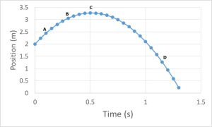
fig-quest3.5 [Image Description]
1. What point(s), (A, B, C, D) represents the instant the object moving in the positive direction? Explain.
2. What point(s), (A, B, C, D) represents the instant the object is moving the fastest? Explain.
3. What point(s), (A, B, C, D) represents the instant the velocity is zero? Explain.
4. Draw a motion diagram representing the motion from point A to point D. Mark point C on the motion diagram.
5. Sketch a velocity vs time graph for the time interval from point A to point D.
Consider the following velocity vs time graph for an object moving along a straight line.

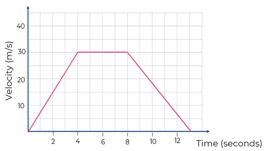
fig-quest3.6 [Image Description]
1. Draw a motion diagram for the time interval from 0s to 4s.
2. Draw a motion diagram for the time interval from 4s to 8s.
3. Draw a motion diagram for the time interval from 8s to 13s.

Problems

[openstax univ. phys. vol1 – 3.38] Dr. John Paul Stapp was a U.S. Air Force officer who studied the effects of extreme acceleration on the human body. On December 10, 1954, Stapp rode a rocket sled, accelerating from rest to a top speed of 282 m/s (1015 km/h) in 5.00 s, and was brought jarringly back to rest in only 1.40 s.
1. Calculate the magnitude of his acceleration while speeding up.
2. Calculate the magnitude of his acceleration while slowing down. Express each in multiples of g (9.80 m/s²) by taking its ratio to the acceleration of gravity.
An object moving along a straight line with constant acceleration passes the origin (x=0) at t=0. In each case determine the position and velocity at t=5.0s and draw a motion diagram to show the motion from t=0s to t=5.0s.
1. The initial velocity is +4.0m/s and the acceleration is -2.0m/s².
2. The initial velocity is -4.0m/s and the acceleration is -2.0m/s².
3. The initial velocity is +4.0m/s and the acceleration is +2.0m/s².
4. The initial velocity is -4.0m/s and the acceleration is +2.0m/s².
5. The initial velocity is +4.0m/s and the acceleration is 0m/s².
In the previous problem, determine the average velocity and the average speed from t=0s to t=5.0s for each case.
[openstax univ. phys. vol1 – 3.49-modified] An object is moving along a straight line with constant acceleration. At t = 10 s, the object is moving from left to right with a speed of 5.0 m/s. At t = 20 s, the particle is moving right to left with a speed of 8.0 m/s. Determine its acceleration.
[openstax univ. phys. vol1 – 3.52] A light-rail commuter train accelerates at a rate of 1.35 m/s².
1. How long does it take to reach its top speed of 80.0 km/h, starting from rest?
2. The same train ordinarily slows down at a rate of 1.65 m/s². How long does it take to come to a stop from its top speed?
3. In emergencies, the train can slow down more rapidly, coming to rest from 80.0 km/h in 8.30 s. What is its emergency acceleration in meters per second squared?
The following is the graph of position vs time for an object moving along a straight line with constant acceleration. Use the graph to answer the following questions.

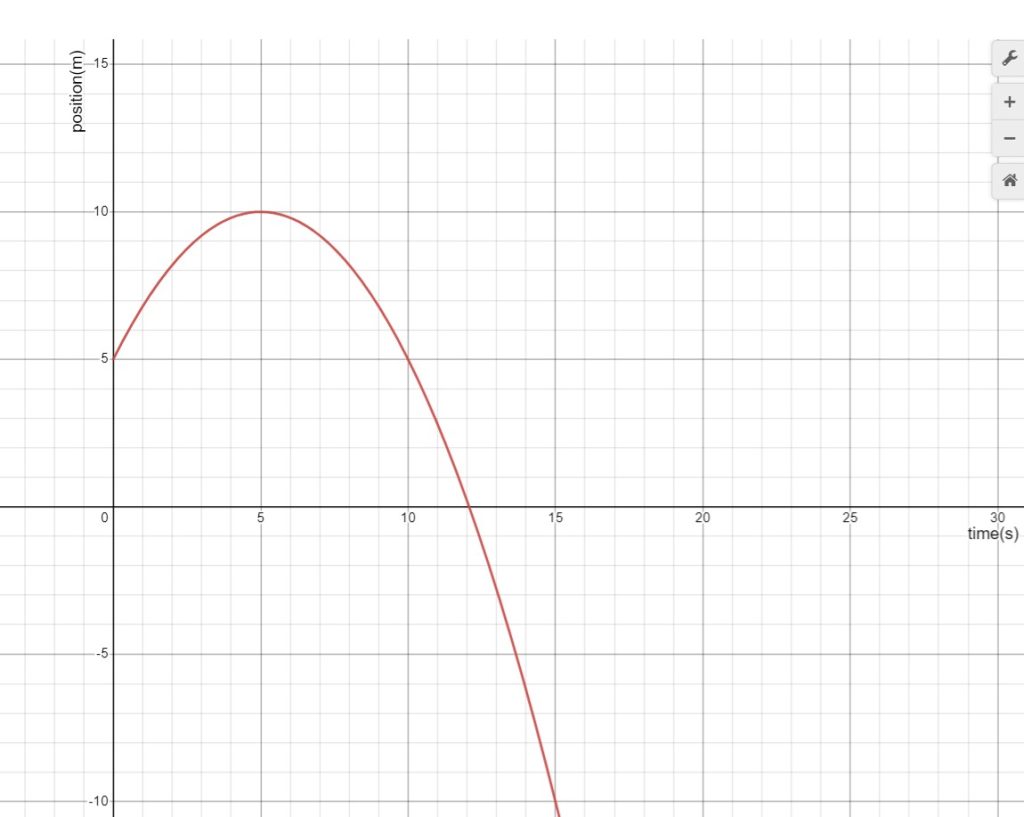
fig-prob3.6 [Image Description]
1. In what direction is the object moving and is the object speeding up, slowing down, or moving with constant velocity from 0s to 5s? from 5s to 15s?
2. Determine the initial velocity of the object (velocity at t=0s), and its velocity at t=8s. Hint: you have to print the graph and use a ruler.
3. At what instant is the velocity zero?
4. Determine the acceleration of this object.
5. Plot the graph of velocity vs time.
6. Draw a motion diagram for this object from t=0s to t=15s.
The following is the graph of position vs time for an object moving along a straight line with constant acceleration. Use the graph to answer the following questions.

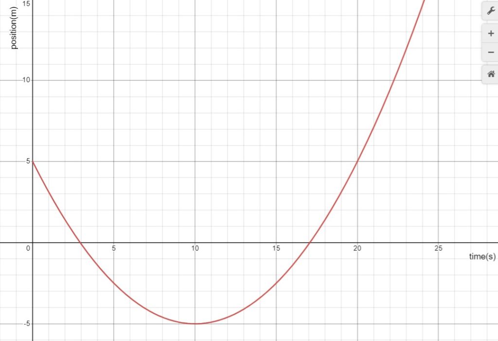
fig-prob3.7 [Image Description]
1. In what direction is the object moving and is the object speeding up, slowing down, or moving with constant velocity from 0s to 10s? from 10s to 24s?
2. Determine the initial velocity of the object (velocity at t=0s), and its velocity at t=15s. Hint: you have to print the graph and use a ruler.
3. At what instant is the velocity zero?
4. Determine the acceleration of this object.
5. Plot the graph of velocity vs time.
6. Draw a motion diagram for this object from t=0s to t=24s.
The following is the graph of velocity vs time for an object moving along a straight line with constant acceleration.

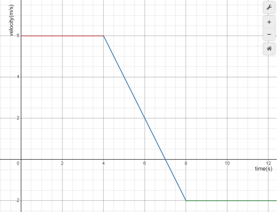
fig-prob3.8 [Image Description]
1. During what time interval(s) is the object moving in the positive direction? in the negative direction?
2. During what time interval(s) is the object slowing down? Speeding up?
3. At what instant does the object change direction? What is the velocity at that moment?
4. What is the acceleration of the object from 0s to 4s? from 4s to 8s?and from 8s to 12s?
[openstax univ. phys. vol1 – 3.39-modified] Consider the following graph of velocity vs time for an object moving along a straight line. Determine the following for each segment of the graph.
1. Is the object moving in the positive direction, moving in the negative direction, or remaining stationary?
2. Is the object speeding up, slowing down, or moving with constant velocity?
3. What is the acceleration of the object?
4. Draw a motion diagram.
5. Sketch the acceleration-versus-time graph for the entire motion from 0s to 100s.
  
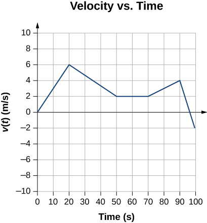
  fig-prob3.9 [Image Description]
A person drops a rock into the water while standing on Verrazano Narrows Bridge in New York City from a height of 72.0m above the water.
1. Find the velocity of the rock after 2.00s.
2. How far is the rock above the water at 2.00s after being released?
3. If the rock was thrown down with a speed of 5.00m/s, how far would it be above the water after 2.00s?
[openstax univ. phys. vol1 – 3.71] A diver bounces straight up from a diving board, avoiding the diving board on the way down, and falls feet first into a pool. She starts with a velocity of 4.00 m/s and her takeoff point is 1.80 m above the pool.
1. What is her highest point above the water?
2. How long a time are her feet in the air?
3. What is her velocity when her feet hit the water?
[openstax univ. phys. vol1 – 3.72] It takes 2.35 s for a rock to hit the ground when it is thrown straight up from the cliff with an initial velocity of 8.00 m/s.
1. Calculate the height of a cliff.
2. How long a time would it take to reach the ground if it is thrown straight down with the same speed?
[openstax univ. phys. vol1 – 3.73] A very strong, but inept, shot putter puts the shot straight up vertically with an initial velocity of 11.0 m/s. How long a time does he have to get out of the way if the shot was released at a height of 2.20 m and he is 1.80 m tall?
[openstax univ. phys. vol1 – 3.74] You throw a ball straight up with an initial velocity of 15.0 m/s. It passes a tree branch on the way up at a height of 7.0 m above the release point. How much additional time elapses before the ball passes the tree branch on the way back down?
[Jeffrey Schnick-SAC106] A car moves along a straight road with constant acceleration. At time 0, the car is 122 m ahead of the start line and moving forward at 80.0 km/h. 5.00 seconds later, the car is 398 m ahead of the start line.
1. Find the acceleration of the car. After you calculate your answer, state your answer by giving a magnitude (a positive value with units) and a direction (write the word “forward” or the word “backward”).
2. Find the velocity of the car at time t = 5.00 State your answer by giving a magnitude and a direction.
[Jeffrey Schnick-SAC106] A train travels along a straight track at a constant acceleration of 0.550 m/s². At the start of observations, the train is already moving forward at 15.0 m/s and the nose of the engine is already 826 m past a railroad crossing sign that you, as an observer, are using as a reference position. How fast is the train going when the nose of the engine is 1.00 km past the same sign?
[Jeffrey Schnick-SAC106A] A boy throws a rock straight upward. The rock leaves the boy’s hand at a point that is 1.40 m above ground level. The maximum altitude achieved by the rock is 10.3 m.
1. How fast is the rock going when it leaves the boy’s hand?
2. How long does it take (starting at the instant when the rock leaves the boy’s hand) for the rock to achieve its maximum altitude?
3. What is the total time of flight of the rock? (The time of flight is the duration of the time interval starting at the instant when the rock is released from the boy’s hand and ending at the instant the rock hits the ground.)
4. How fast is the rock going when it hits the ground (at the instant the rock first makes contact with the ground but before the ground has caused any decrease in the speed of the rock)?

Additional questions and problems

Additional questions and problems related to motion with constant acceleration are available online.

image Descriptions

fig-quest3.5 image description – The image is a graph of position vs time in the shape of a parabola opening down. Points A and B are to the left of the peak, with A being lower than B. The peak is marked with point C. Point D is to the right of the peak and below point A. [Return to the image]

fig-quest3.6 image description – The image is a plot of velocity vs time. The graph consists of three line segments. The first line is from (0s, 0m/s)to (4s, 30m/s). The second line segment is horizontal at 30m/s from 4s to 8s. The last line segment is from (8s, 30m/s) to (13s, 0m/s).[Return to the image]

fig-prob3.6 image description – The image is a plot of position vs time. The position axis is from -10m to 15m, and the time axis is from 0 to 30s. The shape is a parabola opening down. The parabola starts at (0s, 5m), peaks at (5s, 10m), crosses the time axis at 12s, and ends at (15s, -10m). [Return to the image]

fig-prob3.7 image description – The image is a plot of position vs time. The position axis is from -5m to 15m, and the time axis is from 0 to 25s. The shape is a parabola opening up. The parabola starts at (0s, 5m), crosses the time axis at t=3s, the lowest point is at (10s, -5m), crosses the time axis at 17s, and ends at (24s, 15m). [Return to the image]

fig-prob3.8 image description – The image is a plot of velocity vs time. The velocity axis is from -2m/s to 6m/s, and the time axis is from 0 to 12s. The graph consists of three segments. From 0s to 4s, the graph is a horizontal line at 6m/s. From 4s to 8, the graph is a straight line with a negative slope starting at (4s, 6m) and ending at (8s, -2m). From 8s to 12s, the graph is a horizontal line at -2m.[Return to the image]

fig-prob3.9 image description – The image is a plot of velocity vs time. The velocity axis is from -10m/s to 10m/s, and the time axis is from 0 to 100s. The graph consists of five straight-line segments. The first segment starts at (0s, 0m/s) and ends at (20s, 6m/s). the next one starts at (20s, 6m/s) and ends at (50s, 2m/s). The next one is a horizontal line at 2m/s from 50s to 70s. The next one starts at (70s, 2m/s) and ends at (90s, 4m/s). The last one starts at (90s, 4m/s) and ends at (100s, -2m/s)[Return to the image]

License

Icon for the Creative Commons Attribution-NonCommercial-ShareAlike 4.0 International License

Acceleration

average Acceleration

Instantaneous Acceleration

Representation of motion with constant acceleration

Equations of motion

Kinematics Equations

Graphs

Free fall motion

Attributions

Questions and problems

questions

Problems

Additional questions and problems

image Descriptions

License

Share This Book