13.8 The Term Structure of Interest Rates: Four Yield Curve Theories
Here we shall present four theories that attempt to explain why the Yield Curve may take on one or another slope – upward (positive), flat, or downward (negative). We cannot say that any one theory is more correct than the other, nor can we necessarily reconcile one theory in terms of another. Still, the following theories are eminently informative.
1. Pure Expectations – The Market Yield reflects the average of future short-term rates.
First, we assume that investors think about the future and, specifically about the future direction of short-term interest rates. In this notion, we say that the observed Yield Curve is, in a sense, secondary to what market players believe – in their minds – future short-term yields will be. If, as in the mathematical example below, market participants believe that future short-term yields will go higher and higher, then the observed yield curve will reflect this collective belief and be positive in slope – and vice versa. In other words, the Yield Curve reflects market participants’ a priori beliefs.
What makes this interesting is that while we can directly observe the Yield Curve – after all, it is quoted in the media, and by traders and brokers – it is first the unexpressed thoughts and beliefs about the direction of future short-term rates that determine the Yield Curve’s openly expressed slope. We know what is in the public’s minds regarding the future by observing the effect of their collective thought on the slope and shape of the “Yield Curve.” The Yield Curve expresses what people think about the future!
Similarly, the observed Yield Curve – mathematically – will express the average of market participants’ expectations about the course of future short-term rates. For example, standing here today, in the here and now, and assuming first that the investor’s horizon is two years, the investor is faced with two choices: (1) Buy a two-year bond, or (2) Buy a one-year bond and “roll it over” for another year when it comes due at the end of the first year.
Given this line of thinking, if his horizon is three years, an investor can buy a three-year bond, or choose to consecutively roll it over twice. If we assume initially that the two choices in each case should be and are equivalent, we can extrapolate the investor’s beliefs about the “Spot Curve,” i.e., the market’s collective belief about future short-term rates, from the Yield Curve, working backwards. Let’s clarify by mathematical illustration.
Here is an example of how we may calculate “Spot Rates,” or the “Spot Curve” given the Yield Curve (“Market Y-T-M”).
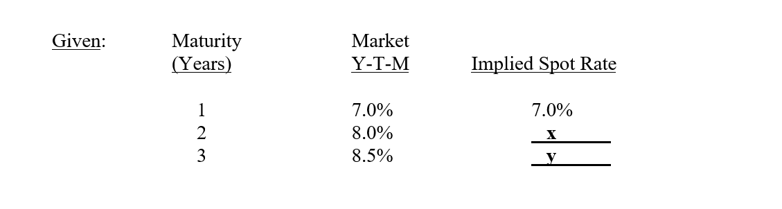
Question:
“x” and “y” represent the future short-term rates that market players anticipate. Specifically, “x” represents the rate for the second period. Likewise, “y” represents the rate for the third period. Working backwards from the observed Yield Curve, what are the values for the two unknowns? Again, we must assume that the two alternatives are equivalent. This mathematical process, by the way, is referred to as “Boot Strapping.”
Solution:
(1.08)2 = (1 + .07) (1 + x)
x = .09009 where, x = 2r1 (i.e., the one-year rate in the second year)
The two alternatives – that of buying (or lending) a two-year instrument or buying (or lending) a one-year instrument and rolling it over at the end of the first year – must be viewed as equivalent alternatives if this idea were to work. And it does because should one alternative be superior, rational, smart market players would go for that one, and the market’s efficient self-correcting mechanism would drive the alternatives together.
This is known as the Law of One Price. This “law” says that if two equal alternatives are present, they must offer the same price or, in this case, yield. If one of the choices were more attractive, investors would choose that one, driving up the price and lowering the yield. They would sell the other, which would have, in the end, an equal and opposite effect. While we have used here the term “investors,” this argument refers to the activities of both borrowers and lenders, in fact.
You should be able to draw these two curves (i.e., both the YTM Yield Curve and Spot Curve, given the calculated values of “x” and “y”) on a chart, with the yield on the vertical and the years-to-maturity on the horizontal. Note that after the first year, the two curves diverge, with the Spot Curve, in this example, rising above the Yield Curve, pulling it upward. Investors expect future, short-term rates to increase! Of course, if the Yield Curve is inverted (negatively sloped), the spot curve would be lower that it and we would conclude that future, short-term rate expectations are decreasing.
As for the nomenclature noted above, and more formally speaking, “2r1” means the “spot rate” starting at the beginning of the second period for the length of one period, while “3r1“starts at the beginning of the third period for one period’s length.
Again, and in summary, why does this math work? This is based on two notions: first, that market players are “rational,” and make optimal decisions that maximize their wealth; second, that markets react “efficiently” to a perceived mispricing should the two opportunities not be equivalent. Together, these two concepts (i.e., Rational Expectations and Efficient Markets) act in unison and cause the alternatives to be equivalent at present. What will actually happen tomorrow is another story.
Under this Pure Expectations Theory, we say that the Yield Curve has no a priori upward (positive) or downward (negative; inverted) bias. The slope of the Yield Curve simply reflects whether people think rates will be going up or down and will acquire its slope accordingly. The observed Yield Curve’s slope thus is a consequence of Pure Expectations.
2. Liquidity Preference – Investors prefer Liquidity to illiquidity.
Investors prefer to be liquid at all times in order to have the freedom to choose whether to spend or invest their funds. Don’t we all want to be free? Should investors choose to tie up their money in an investment, they would demand to be compensated for the illiquidity that comes with investment. Should they tie up their money longer and longer, they would demand that they be increasingly compensated, in terms of higher yield, for their increasing illiquidity. Under this theory, therefore, we conclude that the Yield Curve would have a notable upward bias.
The theories of Pure Expectations and Liquidity Preference are said to work hand-in-hand. When we get both theories working in the same direction, that is, when the Spot Curve is positive, we get a positively sloped Yield Curve. However, if Pure Expectations are such that market participants believe that future short-term rates will decline, the slope will be determined by which force is greater than the other – whether Pure Expectation outweighs Liquidity Preference or not. The following formula expresses this theoretical notion:
(1.07) (1 + x + L) = (1.08)2
While we can measure “x,” i.e., the spot rates, and have just done so, the Liquidity Preferences (L) of the market are not measurable.
There are two more theories to go.
3. Market Segmentation – different segments of the yield curve attract different issuers and investors and are thus subject to varying supply/demand conditions respectively. These conditions will determine the independent slopes of each segment.
In Market Segmentation Theory, we say that participants generally invest or borrow in limited portions or “segments” of the market. Commercial Banks invest very little in the long-term whereas Pension Funds are heavily invested there. Different players tend to “reside” in different “segments.”
Given this segmentation, rates within it would be a function of the supply and demand characteristics of each individual segment, separately and alone. Any changes in a particular maturity’s yield would not affect any other segment, or rate, for any other maturity. There would, thus, be no ex-ante bias whatsoever for the slope of the Yield Curve. In fact, the Yield Curve could conceivably have multiple kinks.
4. Preferred Habitats – Market Segmentation may be altered by yield incentives whereby investors and borrowers may be lured away from their Preferred Habitats.
Preferred Habitats Theory comes to the rescue! Maybe. This theory says that yes, players indeed have their preferred segments, or habitats, but they (i.e., both lenders and borrowers) can be lured away from their preferred habitats if interest rates are attractive enough – low enough for borrowers and high enough for investors.
YOU decide!
