5.5 Liquidity and Liquidity Ratios

We are going to list 20 ratios – covering six categories– in this section. After this discussion, an exercise in calculating all the ratios is presented so that you may apply what you learned.

The first category is liquidity ratios. The idea of liquidity has to do with the ease and speed with which an asset may be converted into cash – without compromising its “true” worth or “intrinsic value.” It must satisfy both conditions in order to be considered liquid. 

For instance, it is possible to sell virtually anything at a “fire–sale price,” if one needs the cash. The question is whether an item worth, say $100, will fetch $100 – or less. If less, we may say that the item is not liquid, as the seller did not obtain its true worth, even though s/he was able to obtain some cash for it.

An example of a liquid asset would be IBM stock. Let’s say it is trading for $190. Should one wish to sell 100 shares of the stock, s/he would obtain approximately $19,000 for it. However, if I wanted to sell my tie, for which I paid $50, it may be difficult for me to get that amount. Whether you wish to consider the asset’s “value” a matter of its original cost or its “current value,” is a matter of analytic choice and context.

The notion of liquidity is closely tied to another notion: “marketability.” This has to do with the availability of a market in which purchases and sales may be readily transacted. For instance, the stock market provides IBM common shares with a great deal of marketability. Should I however wish to sell my tie, I would not know where to go to find a “used-tie market.” Real estate markets are dominated by brokers who advertise frequently, and I may easily sell my car to a used car dealer.

In the case of your typical corporation, it will not own other companies’ stock. It will instead produce goods and services for sale and profit. Thus, it will regularly carry inventory and accounts receivable, which are reported as “current assets.” The net current assets (current assets less current liabilities), being short-term, are presumably liquid. If the assets are liquid, the firm will be able to quickly convert the assets into cash, which will be used to honor its current liabilities due. If not liquid, the firm will have difficulty paying its current liabilities; it will be said to have a “liquidity problem.”

Now that we know what is meant by liquidity and we understand that the liquidity notion applies to “net current assets,” let’s quantify the notion by detailing some relevant ratios that put numbers to the idea. The greater the measurable liquidity the less the risk that the firm will not have sufficient funds to defray its short-term payment requirements.

Current Ratio = Current Assets Divided by Current Liabilities = CA ÷ CL

The current ratio gauges the extent to which a corporation has the liquidity with which it may honor its short-term obligations or liabilities. Does it have the cash to pay its suppliers when accounts payable are due? Are inventories and accounts receivable sufficient (and liquid) to cover its current liabilities? We will assume, for now that the inventory and accounts receivable are completely liquid.

It stands to reason that a watermark level for this ratio should be 1:1 or 1x (“one times”); one would not want to see this ratio go below that figure as it would imply that the company does not have sufficient current assets and, hence, the liquidity to meet its current obligations. Many analysts agree that 1.5x or 2x are reasonable figures, but we should be leery of such arbitrary minima. Companies that are very efficient in the manner in which they manage their current assets may have current ratios close to 1. In general, ratios will vary from industry to industry. Note that this ratio is affected by the choice of inventory costing method (e.g., FIFO vs. LIFO) because inventory is a constituent of current assets.

Some analysts take a more conservative approach in the assessment of liquidity coverage by assuming that inventory is worthless (even though it may, in fact, not be – or not be entirely) and hence that current liabilities will be covered by all current assets except inventory. Indeed, in some industries inventory quickly becomes obsolete due to technological advances; in other cases, inventory may be easily damaged, or lose its fashion and sales appeal.

The current and quick ratios may be thought of as “coverage” ratios in that they indicate the extent to which liquid assets are adequate to “cover,” or pay off, current liabilities, especially accounts payable and notes payable (i.e., short-term loans).

Average Collection Period (ACP) = Days sales outstanding (DSO) = (A/R ÷ Credit Sales) (360)

“A/R” stands for Accounts Receivable. This ratio tells the analyst approximately how long it takes the firm to collect its receivables; the ratio is expressed in days. The shorter the collection period, the more liquid the firm’s accounts receivable.

Note that we use credit sales because only credit (and not cash) sales become accounts receivable. This ACP figure may then be compared to the firm’s typical credit terms. If, for argument’s sake, the ACP exceeds the firm’s credit terms, which may be 30 days, the analyst may first assess whether the firm is having collection problems. Alternatively, the analyst may investigate whether the firm is acting aggressively in its marketing, and choosing to live with the consequences of some late payments as a result. Perhaps the firm expects that the incremental profits will exceed any losses in its collections.

This ratio is our first case, so far, of “apples and oranges” in that, here, we note that both income statement and balance sheet numbers appear within the same ratio. This inconsistency needs to be fixed; we ought not to combine one datum from the Balance Sheet, which is a static figure, with another from the Income Statement, which is a flow kind of number, within one ratio. The two are inconsistent with each other.

In such cases as this, what the analyst may choose to do is “average” the balance sheet number. One way of doing this would be by taking this year’s and last year’s year-end numbers and averaging them(i.e., add the two numbers up and divide by two). We could also use quarterlies or, if available, monthlies. In businesses where receivables fluctuate over the course of the year and may thus be either relatively high or low at certain times of year or during certain seasons, it may be better to average the quarterly numbers, if possible.

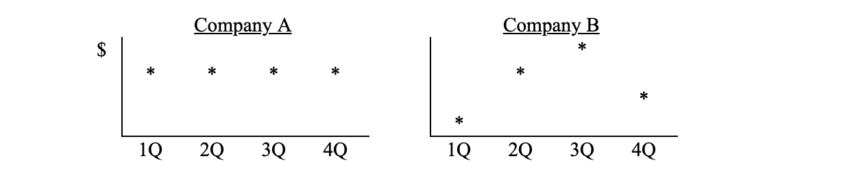
This technique would then capture a better sense of movement over the course of the seasonal business cycle and would thus provide a better comparison with the income statement number, which, again, flow over the course of the entire year. If the balance sheet number does not fluctuate – much, or at all – over time, there may be no need for averaging. This choice is at the discretion of the analyst. Compare Companies “A” and “B” in terms of their accounts receivable or inventory levels, as it were, over the course of four quarters. Is anything accomplished by averaging the Balance Sheet numbers for Company A?

You will also note that (usually) Accounts Receivable will display a smaller number than Sales. Normally, we would expect that accounts receivable are collected more or less monthly; indeed, if sales terms are 30 days, we should get about 12 collections per year. This is illustrated on the next page. 

We shall also assume a 360-day year, consisting of twelve 30-day rolling months, because most often collections are demanded within 30 days. Some analysts will use a 365-day year on the rationale that Credit Sales accumulate over a 365-day calendar year. It’s your choice, Ms/r. Analyst!

Final note: If you are analyzing data for just one quarter, you should use 90, rather than 360, as the multiplier for the ACP. For two or three quarters, you will use 180 and 270 respectively.

Inventory Turnover = COGS ÷ Inventory

This ratio tells us how often the inventory “turns over,” that is to say, how often the inventory – in its entirety – is replaced. Would you buy fresh tomatoes from a company whose inventory turnover is 10x a year (or every 36 days)?  Note that this ratio is affected by the choice of inventory costing method. This ratio has some issues with mixing Balance Sheet and Income Statement numbers, which was discussed the prior section concerning ACP.